Sample: Agriculture, Fresno County: report
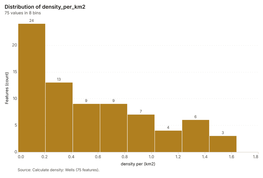
Project: Sample: Agriculture, Fresno County
Goal: Describe the project Sample: Agriculture, Fresno County: run the analyses that tell the most about its data, draw every result, and write a cited report.
Run: 7221484b-d66d-48ff-94e1-dbedfe96dc7c (running, 12 agent run(s))
Generated: 2026-10-18T06:07:57Z, version 1
Model cost: USD 0.0000 over 5 model call(s)
Data used
| Data | Kind | Rows | Time span | Summary | Source |
|---|---|---|---|---|---|
| Fields | vector, Polygon | 60 | 60 polygon (area) features; 'crop' has 5 values (top: tomato 16, almond 16, grape 11); 'irrigation' has 3 values (top: drip 28, micro sprinkler 22, furrow 10); 'area_ha' 43.1 to 43.1 (mean 43.1); 'planted_year' 2,008 to 2,025 (mean 2016); named by 'name' (e.g. Field 001 South, Field 002 South, Field 003 South); total area 25.83 km2; extent -120.0841,36.6269 to -120.0159,36.6731. Areas (Fields) with area_ha to compare and map. | 100 | |
| Satellite scene 2026-04-15 | raster | 2026-04-15 | 4-band float32 raster (imagery), 300 x 250 cells; resolution 20; band 1 0.014 to 0.113; acquired 2026-04-15; extent -120.0844,36.6267 to -120.0156,36.6733. Imagery for visual and change analysis. | 101 | |
| Satellite scene 2026-08-15 | raster | 2026-08-15 | 4-band float32 raster (imagery), 300 x 250 cells; resolution 20; band 1 0.015 to 0.145; acquired 2026-08-15; extent -120.0844,36.6267 to -120.0156,36.6733. Imagery for visual and change analysis. | 102 | |
| Soil samples | vector, Point | 600 | 2025-10-01 to 2026-02-27 | 600 point features; dated by 'sampled_on' from 2025-10-01 to 2026-02-27; 'ph' 6.4 to 9 (mean 7.401); 'organic_matter_pct' 0.11 to 1.99 (mean 1.236); 'nitrate_ppm' 3.6 to 65.5 (mean 17.55); extent -120.0834,36.6274 to -120.0174,36.6729. Dated point events: where and when Soil samples happen. | 2 |
| Irrigation canals | vector, LineString | 5 | 5 line features; 'type' has 2 values (top: lateral 3, canal 2); 'capacity_cfs' 38 to 232 (mean 143); named by 'name' (e.g. Canal 1, Canal 2, Lateral 1); total length 26.99 km; extent -120.0838,36.6270 to -120.0162,36.6730. Lines (Irrigation canals) such as routes or networks. | 103 | |
| Wells | vector, Point | 40 | 40 point features; 'depth_ft' 307 to 871 (mean 604.4); 'pump_hp' 75 to 200 (mean 140.6); 'static_level_ft' 120 to 418 (mean 282.7); extent -120.0823,36.6281 to -120.0188,36.6714. Point locations of Wells. | 104 | |
| Pest scouting | vector, Point | 520 | 2026-04-01 to 2026-09-14 | 520 point features; dated by 'observed_at' from 2026-04-01 to 2026-09-14; 'pest' has 4 values (top: aphid 235, navel orangeworm 110, lygus 92); 'threshold_exceeded' has 2 values (top: False 374, True 146); 'count_per_trap' 0 to 13 (mean 4.477); extent -120.0833,36.6271 to -120.0169,36.6728. Dated point events by pest: where and when Pest scouting happen. | 3 |
| Weather stations | vector, Point | 3 | 3 point features; 'elevation_m' 57 to 65 (mean 61.67); named by 'name' (e.g. Farm weather station 1, Farm weather station 2, Farm weather station 3); extent -120.0663,36.6367 to -120.0366,36.6639. Point locations of Weather stations. | 105 | |
| Yields by season | table | 300 | 2021-01-01 to 2025-01-01 | Table of 300 rows and 5 columns without geometry; dated by 'season' from 2021-01-01 to 2025-01-01; 'crop' has 5 values (top: tomato 80, almond 80, grape 55); 'yield_t_ha' 1.19 to 120.7 (mean 33.16); 'water_af_per_acre' 2.6 to 4.2 (mean 3.395). A table of Yields by season without locations. | 4 |
| Field operations | table | 272 | 2026-02-01 to 2026-09-27 | Table of 272 rows and 5 columns without geometry; dated by 'date' from 2026-02-01 to 2026-09-27; 'operation' has 4 values (top: cultivate 74, irrigate 68, spray 67); 'product' has 3 values (top: UAN-32 67, sulfur 65, water 64); 'rate' 5.1 to 59.9 (mean 33.66). A table of Field operations without locations. | 5 |
| Agronomist season notes | document | 1-page md document 'Agronomist season notes, August 2026'; language en; mentions 7 place(s): Field 001 South (1), Field 010 South (1), Field 017 South (1), Field 018 South (1), Field (1). A document about Field 001 South, Field 010 South, Field 017 South. | 106 | ||
| Sample: Agriculture, Fresno County | record | 107 | |||
| Summarize within: Fields | layer, Polygon | 60 | 108 | ||
| Summarize within: Fields | layer, Polygon | 60 | 109 | ||
| Summarize within: Fields | layer, Polygon | 60 | 110 | ||
| Emerging hot spots: Pest scouting | layer, Polygon | 48 | 111 | ||
| Emerging hot spots: Soil samples | layer, Polygon | 51 | 112 | ||
| Repeat and near repeat classification: Pest scouting | layer, Point | 520 | 113 | ||
| NDVI change Satellite scene 2026-04-15 to Satellite scene 2026-08-15 | layer | 0 | 114 | ||
| NDVI decrease / increase | layer | 0 | 115 | ||
| NDVI change polygons | layer, Polygon | 175 | 116 | ||
| Difference Satellite scene 2026-04-15 to Satellite scene 2026-08-15 | layer | 0 | 117 | ||
| Hot spot analysis: Pest scouting | layer, Polygon | 134 | 118 | ||
| Hot spot analysis: Wells | layer, Polygon | 13 | 119 | ||
| Hot spot analysis: Soil samples | layer, Polygon | 139 | 120 | ||
| Calculate density: Pest scouting | layer, Polygon | 937 | 121 | ||
| Calculate density: Wells | layer, Polygon | 75 | 122 | ||
| Calculate density: Soil samples | layer, Polygon | 953 | 123 | ||
| Find point clusters: Pest scouting | layer, Point | 520 | 124 | ||
| Find point clusters: cluster hulls | layer, Polygon | 4 | 125 | ||
| Find point clusters: Wells | layer, Point | 40 | 126 | ||
| Find point clusters: cluster hulls | layer, Polygon | 5 | 127 | ||
| Find point clusters: Soil samples | layer, Point | 600 | 128 |
Timeline
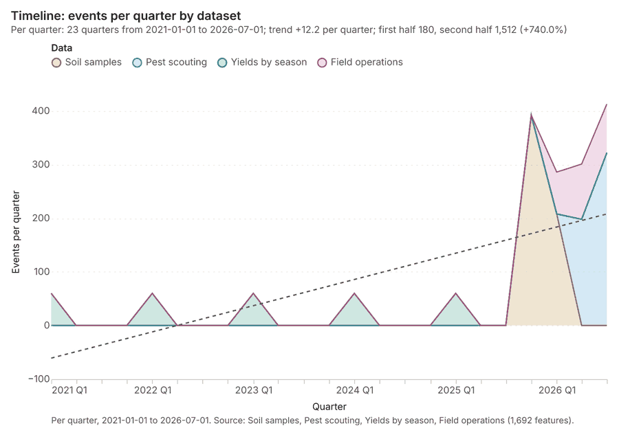
The timeline counts 1,692 dated events in Soil samples, Pest scouting, Yields by season and 1 more per quarter, from Q1 2021 to Q3 2026 12345. By dataset: Soil samples 600; Pest scouting 520; Yields by season 300; Field operations 272 1. The trend is +12.2 events per quarter; the second half of the quarters has 1,512 against 180 in the first (+740.0%) 1. 14 of the 23 quarters had no events 1.
Busiest quarters
Quietest quarters with events
Summarize within
What this analysis is. Summarize within: Count and aggregate the features inside each polygon (or bin), proportionally for lines and polygons 6. In ArcGIS it is Summarize Within or Aggregate Points; in QGIS, native:countpointsinpolygon or native:sumlinelengths 6.
Why it was run on this data. Count Weather stations inside each feature of Fields; the counts map as a choropleth (natural breaks, sequential colors) 7.
What it found. Summarize within on Weather stations, Fields: Summarize within: 1 layer saved: Summarize within: Fields (60 features) 8910. It reported result, count 60; result, elapsed ms 2; billing, cost 0.01128; billing, list price 0.01128; billing, upstream cost 0 8.
| Result | Value |
|---|---|
| result, count | 60 |
| result, elapsed ms | 2 |
| billing, cost | 0.01128 |
| billing, list price | 0.01128 |
| billing, upstream cost | 0 |
Findings
- Evidenced: Summarize within on Weather stations, Fields: Summarize within: 1 layer saved: Summarize within: Fields (60 features) 8910.
- Evidenced: It reported result, count 60; result, elapsed ms 2; billing, cost 0.01128; billing, list price 0.01128; billing, upstream cost 0 8.
Tool gp_summarize_within; parameters {"stats": [{"stat": "sum", "field": "elevation_m"}], "project": "c0ff746c-cbbb-48c5-a026-444453a7b463", "features": {"layer": "Weather stations (7a8242c6)"}, "polygons": {"layer": "Fields (a196eb79)"}}
Summarize within
What this analysis is. Summarize within: Count and aggregate the features inside each polygon (or bin), proportionally for lines and polygons 6. In ArcGIS it is Summarize Within or Aggregate Points; in QGIS, native:countpointsinpolygon or native:sumlinelengths 6.
Why it was run on this data. Count Weather stations inside each feature of Fields; the counts map as a choropleth (natural breaks, sequential colors) 7.
What it found. Summarize within on Pest scouting, Fields: Summarize within: 1 layer saved: Summarize within: Fields (60 features) 101112. It reported result, count 60; result, elapsed ms 2; billing, cost 0.02162; billing, list price 0.02162; billing, upstream cost 0 11.
| Result | Value |
|---|---|
| result, count | 60 |
| result, elapsed ms | 2 |
| billing, cost | 0.02162 |
| billing, list price | 0.02162 |
| billing, upstream cost | 0 |
Findings
- Evidenced: Summarize within on Pest scouting, Fields: Summarize within: 1 layer saved: Summarize within: Fields (60 features) 101112.
- Evidenced: It reported result, count 60; result, elapsed ms 2; billing, cost 0.02162; billing, list price 0.02162; billing, upstream cost 0 11.
Tool gp_summarize_within; parameters {"stats": [{"stat": "sum", "field": "count_per_trap"}], "project": "c0ff746c-cbbb-48c5-a026-444453a7b463", "features": {"layer": "Pest scouting (815c2b2c)"}, "group_by": "pest", "polygons": {"layer": "Fields (a196eb79)"}}
Summarize within
What this analysis is. Summarize within: Count and aggregate the features inside each polygon (or bin), proportionally for lines and polygons 6. In ArcGIS it is Summarize Within or Aggregate Points; in QGIS, native:countpointsinpolygon or native:sumlinelengths 6.
Why it was run on this data. Count Weather stations inside each feature of Fields; the counts map as a choropleth (natural breaks, sequential colors) 7.
What it found. Summarize within on Wells, Fields: Summarize within: 1 layer saved: Summarize within: Fields (60 features) 101314. It reported result, count 60; result, elapsed ms 1; billing, cost 0.01202; billing, list price 0.01202; billing, upstream cost 0 13.
| Result | Value |
|---|---|
| result, count | 60 |
| result, elapsed ms | 1 |
| billing, cost | 0.01202 |
| billing, list price | 0.01202 |
| billing, upstream cost | 0 |
Findings
- Evidenced: Summarize within on Wells, Fields: Summarize within: 1 layer saved: Summarize within: Fields (60 features) 101314.
- Evidenced: It reported result, count 60; result, elapsed ms 1; billing, cost 0.01202; billing, list price 0.01202; billing, upstream cost 0 13.
Tool gp_summarize_within; parameters {"stats": [{"stat": "sum", "field": "depth_ft"}], "project": "c0ff746c-cbbb-48c5-a026-444453a7b463", "features": {"layer": "Wells (15d08948)"}, "polygons": {"layer": "Fields (a196eb79)"}}
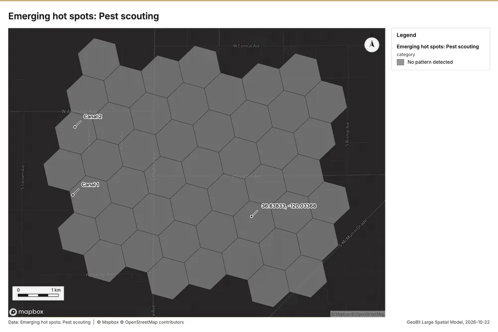
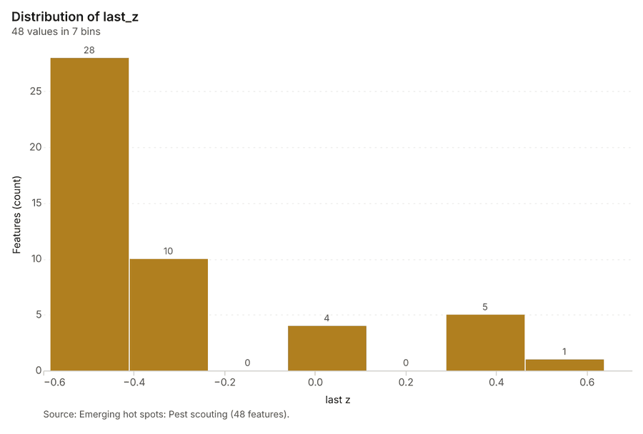
Space time hot spots
What this analysis is. Emerging hot spots: Where hot spots are new, consecutive, intensifying, persistent, diminishing, sporadic, oscillating or historical over time 15. In ArcGIS it is Emerging Hot Spot Analysis or Create Space Time Cube 15.
Why it was run on this data. Pest scouting carry dates in 'observed_at': emerging hot spot analysis finds new, intensifying and fading hot spots per week 16.
What it found. The process began with the "Pest scouting" input 12. Running the "gp_space_time_hot_spots" tool yielded a result containing 48 features 17. This analysis required using 520 features and completed in 8 milliseconds 17. The computational cost for this operation was 0.126 17.
| Result | Value |
|---|---|
| result, count | 48 |
| result, elapsed ms | 8 |
| result, resolution | 8 |
| result, features used | 520 |
| result, time neighbors | 0 |
| billing, cost | 0.126 |
| billing, list price | 0.126 |
| billing, upstream cost | 0 |
Findings
- Evidenced: Space time hot spots on Pest scouting: Emerging hot spots: 1 layer saved: Emerging hot spots: Pest scouting (48 features) 1217.
- Evidenced: It reported result, count 48; result, elapsed ms 8; result, resolution 8; result, features used 520; result, time neighbors 0; billing, cost 0.126 17.
Tool gp_space_time_hot_spots; parameters {"project": "c0ff746c-cbbb-48c5-a026-444453a7b463", "features": {"layer": "Pest scouting (815c2b2c)"}, "interval": "week", "bin_shape": "h3", "resolution": 8, "time_field": "observed_at"}
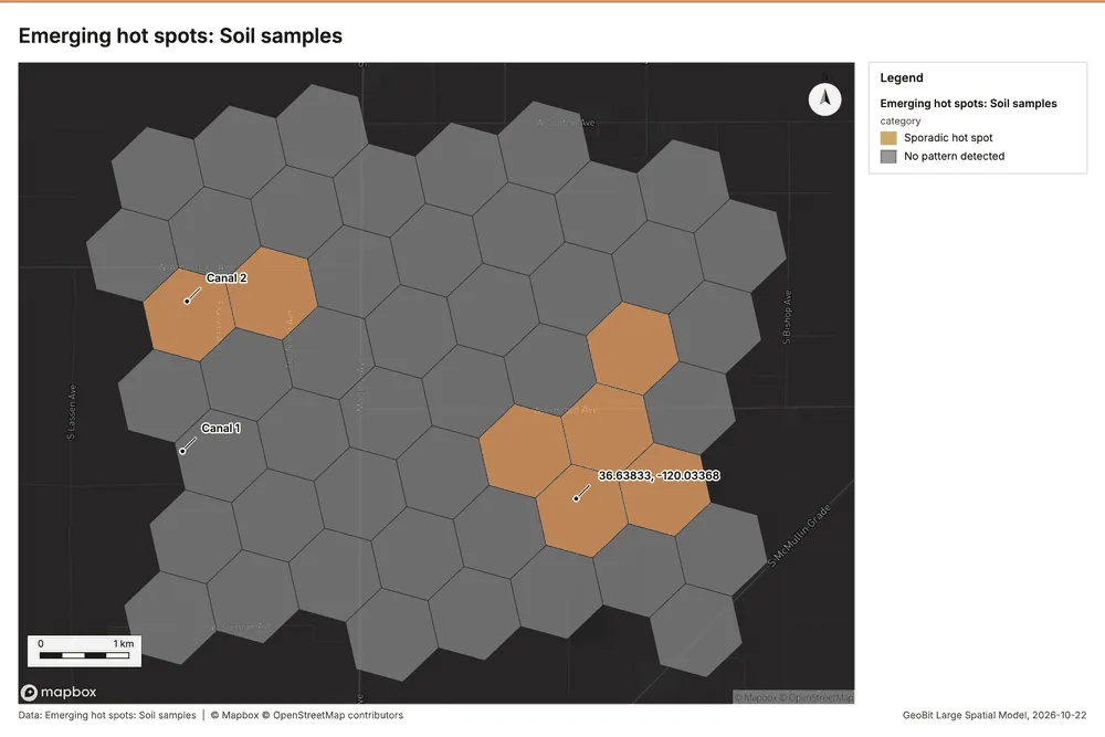
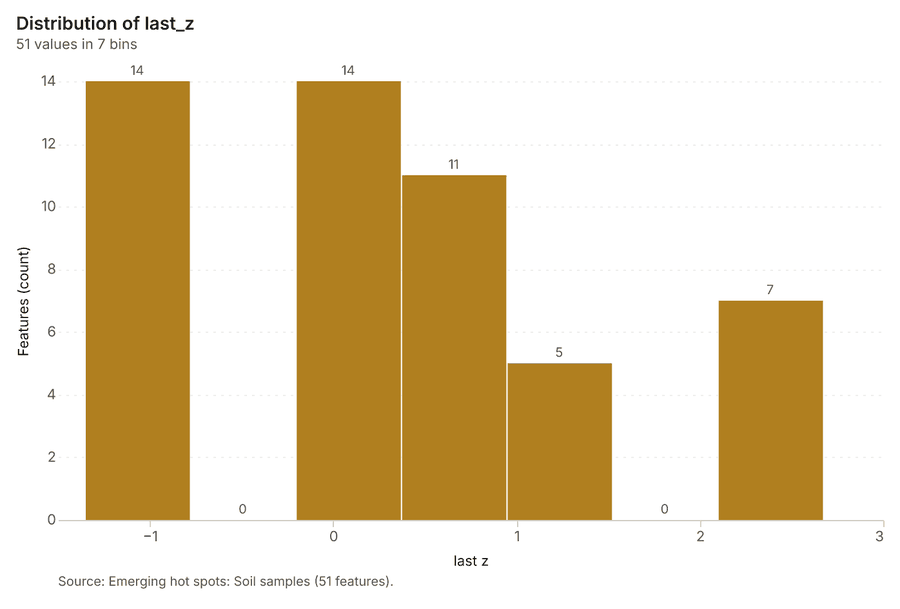
Space time hot spots
What this analysis is. Emerging hot spots: Where hot spots are new, consecutive, intensifying, persistent, diminishing, sporadic, oscillating or historical over time 15. In ArcGIS it is Emerging Hot Spot Analysis or Create Space Time Cube 15.
Why it was run on this data. Soil samples carry dates in 'sampled_on': emerging hot spot analysis finds new, intensifying and fading hot spots per week 18.
What it found. The analysis processed the Soil samples 20 and resulted in 51 emerging
| Result | Value |
|---|---|
| result, count | 51 |
| result, elapsed ms | 8 |
| result, resolution | 8 |
| result, features used | 600 |
| result, time neighbors | 0 |
| billing, cost | 0.13 |
| billing, list price | 0.13 |
| billing, upstream cost | 0 |
Findings
- Evidenced: Space time hot spots on Soil samples: Emerging hot spots: 1 layer saved: Emerging hot spots: Soil samples (51 features) 1920.
- Evidenced: It reported result, count 51; result, elapsed ms 8; result, resolution 8; result, features used 600; result, time neighbors 0; billing, cost 0.13 19.
Tool gp_space_time_hot_spots; parameters {"project": "c0ff746c-cbbb-48c5-a026-444453a7b463", "features": {"layer": "Soil samples (caf67b23)"}, "interval": "week", "bin_shape": "h3", "resolution": 8, "time_field": "sampled_on"}
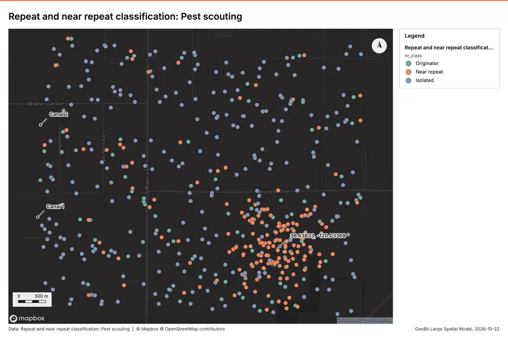
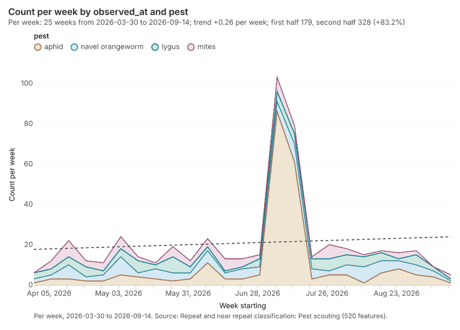
Near repeat
What this analysis is. Repeat and near repeat classification: Classify incidents as originators, repeats (same place) or near repeats within a distance and time window, with a Knox test table 21. In ArcGIS it is Repeat and Near Repeat Classification or Near Repeat Calculator 21.
Why it was run on this data. Near repeat analysis tests whether Pest scouting close in space also follow each other within 17 days 22.
What it found. Near repeat on Pest scouting: Repeat and near repeat classification: 1 layer saved: Repeat and near repeat classification: Pest scouting (520 features) 1223. It reported result, days 17; result, count 520; result, chains 48; result, distance m 200; result, elapsed ms 11; result, pairs linked 529 23.
| Result | Value |
|---|---|
| result, days | 17 |
| result, count | 520 |
| result, chains | 48 |
| result, distance m | 200 |
| result, elapsed ms | 11 |
| result, pairs linked | 529 |
| billing, cost | 0.0656 |
| billing, list price | 0.0656 |
| billing, upstream cost | 0 |
Findings
- Evidenced: Near repeat on Pest scouting: Repeat and near repeat classification: 1 layer saved: Repeat and near repeat classification: Pest scouting (520 features) 1223.
- Evidenced: It reported result, days 17; result, count 520; result, chains 48; result, distance m 200; result, elapsed ms 11; result, pairs linked 529 23.
Tool gp_near_repeat; parameters {"days": 17, "project": "c0ff746c-cbbb-48c5-a026-444453a7b463", "features": {"layer": "Pest scouting (815c2b2c)"}, "distance_m": 200.0, "time_field": "observed_at"}
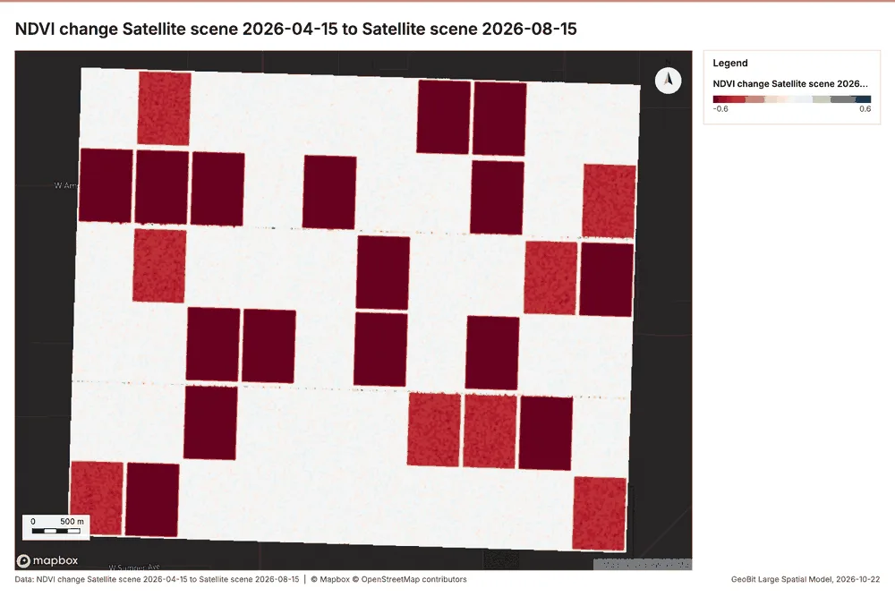
Index change
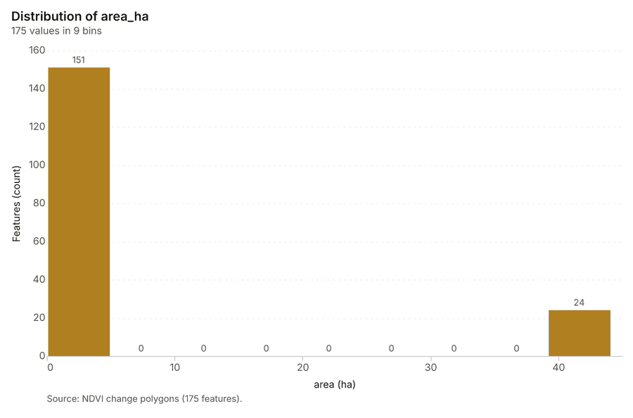
What this analysis is. Spectral index change: Change of a spectral index (NDVI, NDWI, NDBI, NBR …) or a band expression between two images: before, after and difference rasters, decrease / increase classes beyond the threshold with polygons and areas; NBR also gives dNBR with burn severity classes 24.
Why it was run on this data. Index change between Satellite scene 2026-04-15 (2026-04-15) and Satellite scene 2026-08-15 (2026-08-15): the changed area, with the changed places as polygons 25.
What it found. Index change: Spectral index change: created NDVI change Satellite scene 2026-04-15 to Satellite scene 2026-08-15 (300 x 250 cells, 20.00 m) 26. plus 1 more raster layer(s) 26. and layer NDVI change polygons with 175 feature(s) 26. mean before 0.7068; mean after 0.5038; mean difference -0.203; decrease ha 1,053; increase ha 5.32 26. It reported stats, polygons 175; stats, mean after 0.5038; stats, decrease ha 1,053; stats, increase ha 5.32; stats, mean before 0.7068; stats, masked pixels 0 26.
| Result | Value |
|---|---|
| stats, polygons | 175 |
| stats, mean after | 0.5038 |
| stats, decrease ha | 1,053 |
| stats, increase ha | 5.32 |
| stats, mean before | 0.7068 |
| stats, masked pixels | 0 |
| stats, mean difference | -0.203 |
| elapsed ms | 175 |
Findings
- Evidenced: Index change: Spectral index change: created NDVI change Satellite scene 2026-04-15 to Satellite scene 2026-08-15 (300 x 250 cells, 20.00 m) 26.
- Evidenced: plus 1 more raster layer(s) 26.
- Evidenced: and layer NDVI change polygons with 175 feature(s) 26.
- Evidenced: mean before 0.7068; mean after 0.5038; mean difference -0.203; decrease ha 1,053; increase ha 5.32 26.
- Evidenced: It reported stats, polygons 175; stats, mean after 0.5038; stats, decrease ha 1,053; stats, increase ha 5.32; stats, mean before 0.7068; stats, masked pixels 0 26.
Tool im_index_change; parameters {"after_id": "Satellite scene 2026-08-15 (34efa462)", "polygons": true, "before_id": "Satellite scene 2026-04-15 (6c1f22ed)"}
Compute change raster
What this analysis is. Compute change raster: Pixel value or spectral change between two co-registered images: difference, relative difference, absolute difference, log ratio (radar, dB), Euclidean spectral distance, spectral angle (radians) or the band with most change 27.
Why it was run on this data. A change raster between Satellite scene 2026-04-15 (2026-04-15) and Satellite scene 2026-08-15 (2026-08-15): where and how much the pixels changed 28.
What it found. Compute change raster: Compute change raster: created Difference Satellite scene 2026-04-15 to Satellite scene 2026-08-15 (300 x 250 cells, 20.00 m) 29. mean 0.02217; std 0.03434; min -0.037; max 0.116; masked pixels 0 29. It reported stats, max 0.116; stats, min -0.037; stats, std 0.03434; stats, mean 0.02217; stats, masked pixels 0; elapsed ms 88 29.
| Result | Value |
|---|---|
| stats, max | 0.116 |
| stats, min | -0.037 |
| stats, std | 0.03434 |
| stats, mean | 0.02217 |
| stats, masked pixels | 0 |
| elapsed ms | 88 |
Findings
- Evidenced: Compute change raster: Compute change raster: created Difference Satellite scene 2026-04-15 to Satellite scene 2026-08-15 (300 x 250 cells, 20.00 m) 29.
- Evidenced: mean 0.02217; std 0.03434; min -0.037; max 0.116; masked pixels 0 29.
- Evidenced: It reported stats, max 0.116; stats, min -0.037; stats, std 0.03434; stats, mean 0.02217; stats, masked pixels 0; elapsed ms 88 29.
Tool im_compute_change_raster; parameters {"after_id": "Satellite scene 2026-08-15 (34efa462)", "before_id": "Satellite scene 2026-04-15 (6c1f22ed)"}
Hot spots
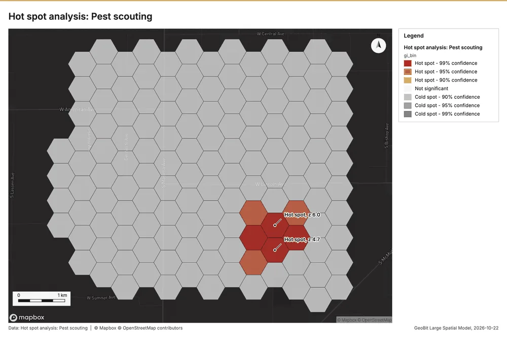
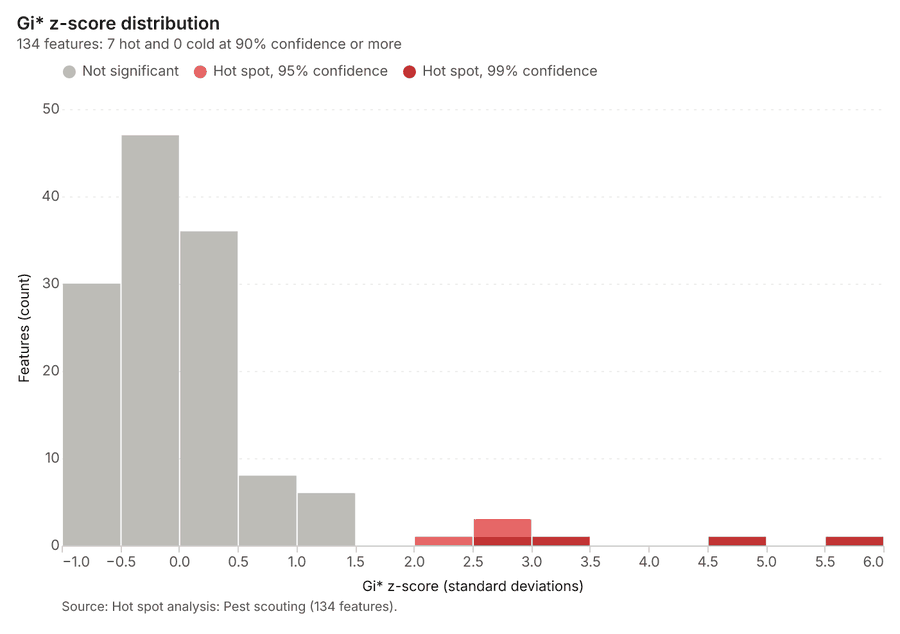
What this analysis is. Hot spot analysis: Getis-Ord Gi* hot and cold spots with z-scores, p-values and confidence bins 30. In ArcGIS it is Find Hot Spots or Hot Spot Analysis (Getis-Ord Gi*); in QGIS, qgis:hotspot (plugin) 30.
Why it was run on this data. 520 points: Getis-Ord Gi* tests whether the concentrations in Pest scouting are statistically significant 31.
What it found. Hot spots on Pest scouting: Hot spot analysis: 1 layer saved: Hot spot analysis: Pest scouting (134 features) 1232. It reported result, bins 134; result, count 134; result, elapsed ms 10; result, cell size m 500; result, incidents used 520; result, distance band m 500 32.
| Result | Value |
|---|---|
| result, bins | 134 |
| result, count | 134 |
| result, elapsed ms | 10 |
| result, cell size m | 500 |
| result, incidents used | 520 |
| result, distance band m | 500 |
| billing, cost | 0.0604 |
| billing, list price | 0.0604 |
| billing, upstream cost | 0 |
Findings
- Evidenced: Hot spots on Pest scouting: Hot spot analysis: 1 layer saved: Hot spot analysis: Pest scouting (134 features) 1232.
- Evidenced: It reported result, bins 134; result, count 134; result, elapsed ms 10; result, cell size m 500; result, incidents used 520; result, distance band m 500 32.
A model draft was discarded because a sentence did not cite a source of this section.
Tool gp_hot_spots; parameters {"project": "c0ff746c-cbbb-48c5-a026-444453a7b463", "features": {"layer": "Pest scouting (815c2b2c)"}, "aggregation": "hexagon", "cell_size_m": 500.0, "distance_band_m": 500.0}
Hot spots
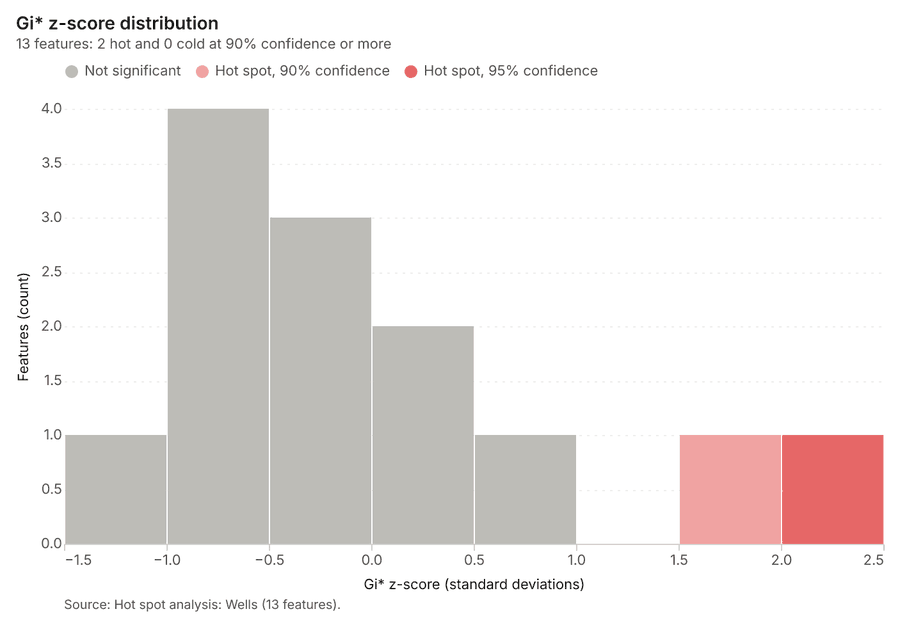
What this analysis is. Hot spot analysis: Getis-Ord Gi* hot and cold spots with z-scores, p-values and confidence bins 30. In ArcGIS it is Find Hot Spots or Hot Spot Analysis (Getis-Ord Gi*); in QGIS, qgis:hotspot (plugin) 30.
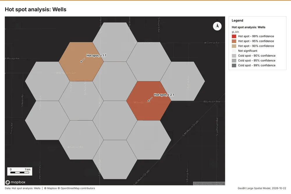
Why it was run on this data. 40 points: Getis-Ord Gi* tests whether the concentrations in Wells are statistically significant 33.
What it found. The utilization of the Hot spot analysis tool (gp_hot_spots) processed the Wells data 14. The analysis yielded a saved layer with 13 features 34. Performance metrics showed that the analysis involved 13 bins, counted 13 results, and took 2 elapsed ms 34.
| Result | Value |
|---|---|
| result, bins | 13 |
| result, count | 13 |
| result, elapsed ms | 2 |
| result, cell size m | 2,000 |
| result, incidents used | 40 |
| result, distance band m | 2,000 |
| billing, cost | 0.0508 |
| billing, list price | 0.0508 |
| billing, upstream cost | 0 |
Findings
- Evidenced: Hot spots on Wells: Hot spot analysis: 1 layer saved: Hot spot analysis: Wells (13 features) 1434.
- Evidenced: It reported result, bins 13; result, count 13; result, elapsed ms 2; result, cell size m 2,000; result, incidents used 40; result, distance band m 2,000 34.
Tool gp_hot_spots; parameters {"project": "c0ff746c-cbbb-48c5-a026-444453a7b463", "features": {"layer": "Wells (15d08948)"}, "aggregation": "hexagon", "cell_size_m": 2000.0, "distance_band_m": 2000.0}
Hot spots
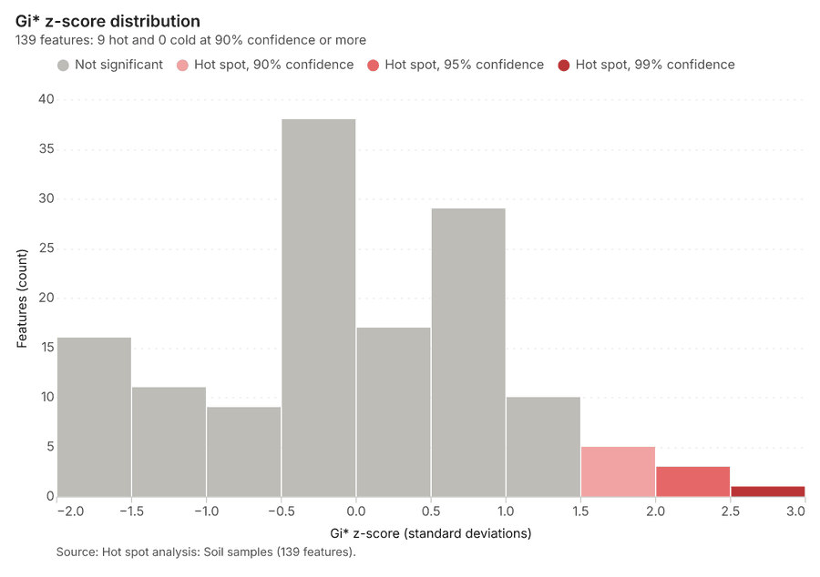
What this analysis is. Hot spot analysis: Getis-Ord Gi* hot and cold spots with z-scores, p-values and confidence bins 30. In ArcGIS it is Find Hot Spots or Hot Spot Analysis (Getis-Ord Gi*); in QGIS, qgis:hotspot (plugin) 30.
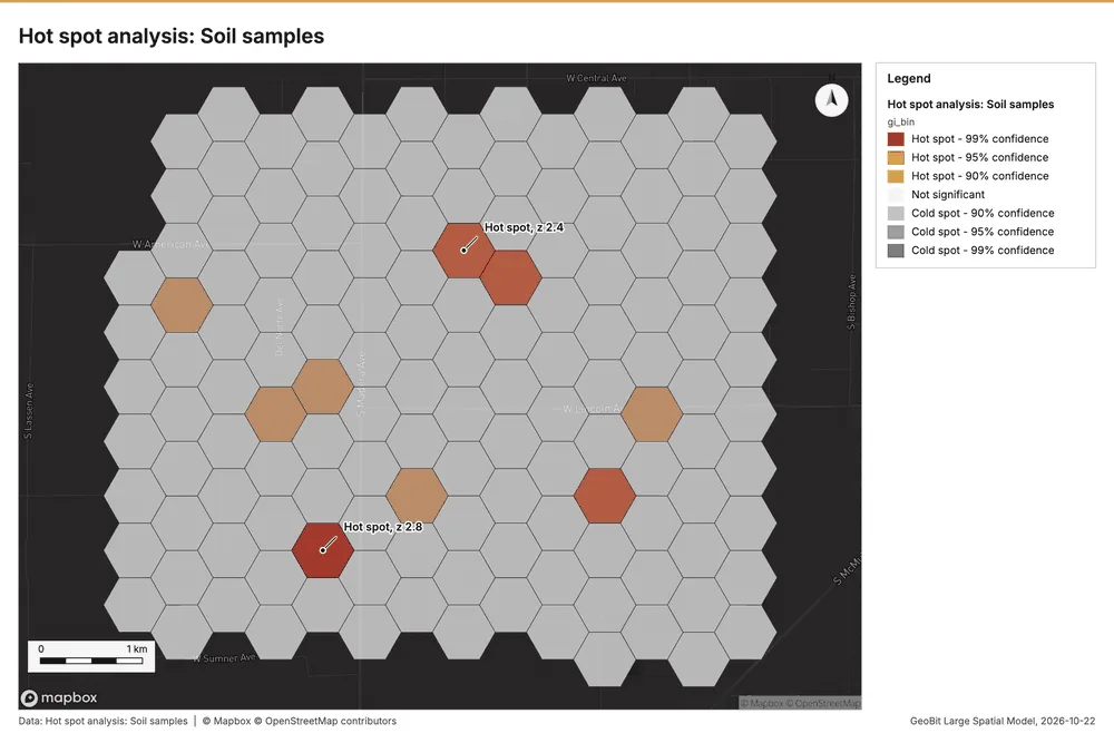
Why it was run on this data. 600 points: Getis-Ord Gi* tests whether the concentrations in Soil samples are statistically significant 35.
What it found. Hot spots on Soil samples: Hot spot analysis: 1 layer saved: Hot spot analysis: Soil samples (139 features) 2036. It reported result, bins 139; result, count 139; result, elapsed ms 10; result, cell size m 500; result, incidents used 600; result, distance band m 500 36.
| Result | Value |
|---|---|
| result, bins | 139 |
| result, count | 139 |
| result, elapsed ms | 10 |
| result, cell size m | 500 |
| result, incidents used | 600 |
| result, distance band m | 500 |
| billing, cost | 0.062 |
| billing, list price | 0.062 |
| billing, upstream cost | 0 |
Findings
- Evidenced: Hot spots on Soil samples: Hot spot analysis: 1 layer saved: Hot spot analysis: Soil samples (139 features) 2036.
- Evidenced: It reported result, bins 139; result, count 139; result, elapsed ms 10; result, cell size m 500; result, incidents used 600; result, distance band m 500 36.
Tool gp_hot_spots; parameters {"project": "c0ff746c-cbbb-48c5-a026-444453a7b463", "features": {"layer": "Soil samples (caf67b23)"}, "aggregation": "hexagon", "cell_size_m": 500.0, "distance_band_m": 500.0}
Calculate density
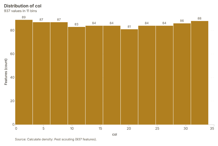
What this analysis is. Calculate density: Kernel density per square kilometer on a grid 37. In ArcGIS it is Calculate Density or Kernel Density; in QGIS, native:heatmapkerneldensityestimation 37.
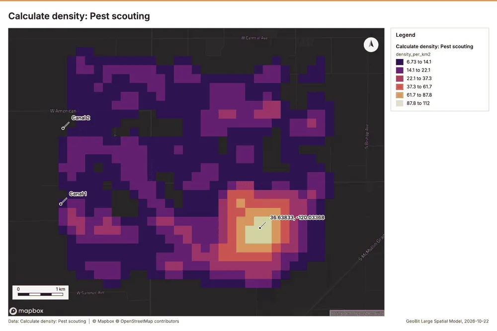
Why it was run on this data. 520 points in Pest scouting: a density surface shows where they concentrate 38.
What it found. Calculate density on Pest scouting: Calculate density: 1 layer saved: Calculate density: Pest scouting (937 features) 1239. It reported result, count 937; result, elapsed ms 41; result, bandwidth m 500; result, cell size m 200; result, excluded null 0; result, max density per km2 111.6 39.
| Result | Value |
|---|---|
| result, count | 937 |
| result, elapsed ms | 41 |
| result, bandwidth m | 500 |
| result, cell size m | 200 |
| result, excluded null | 0 |
| result, max density per km2 | 111.6 |
| billing, cost | 0.0604 |
| billing, list price | 0.0604 |
| billing, upstream cost | 0 |
Findings
- Evidenced: Calculate density on Pest scouting: Calculate density: 1 layer saved: Calculate density: Pest scouting (937 features) 1239.
- Evidenced: It reported result, count 937; result, elapsed ms 41; result, bandwidth m 500; result, cell size m 200; result, excluded null 0; result, max density per km2 111.6 39.
Tool gp_calculate_density; parameters {"kernel": "quartic", "project": "c0ff746c-cbbb-48c5-a026-444453a7b463", "features": {"layer": "Pest scouting (815c2b2c)"}, "bandwidth_m": 500.0, "cell_size_m": 200.0}
Calculate density
What this analysis is. Calculate density: Kernel density per square kilometer on a grid 37. In ArcGIS it is Calculate Density or Kernel Density; in QGIS, native:heatmapkerneldensityestimation 37.
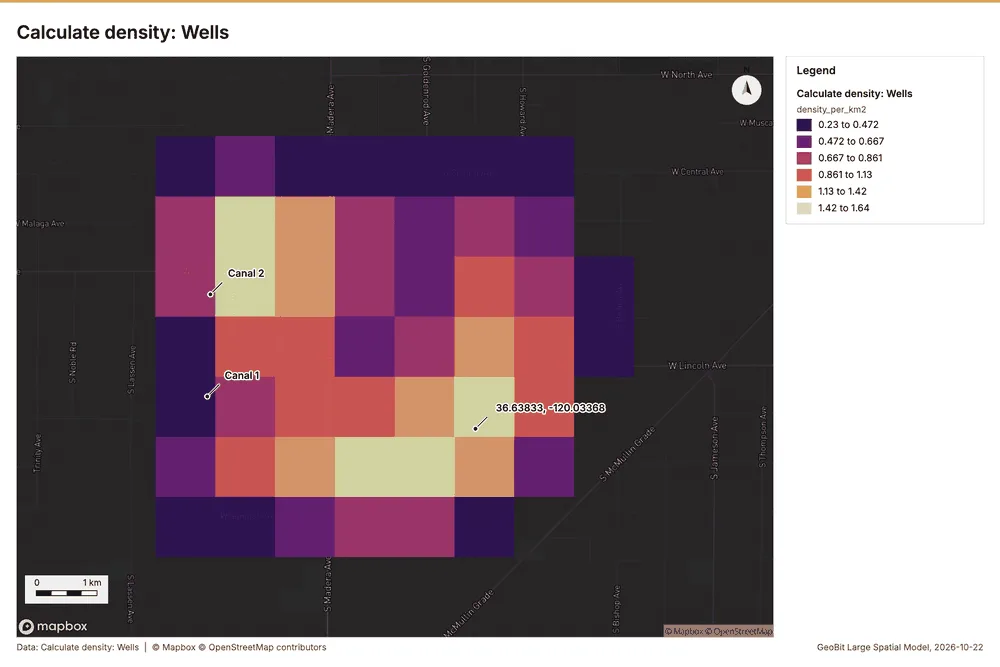
Why it was run on this data. 40 points in Wells: a density surface shows where they concentrate 40.
What it found. Calculate density on Wells: Calculate density: 1 layer saved: Calculate density: Wells (75 features) 1441. It reported result, count 75; result, elapsed ms 3; result, bandwidth m 2,000; result, cell size m 1,000; result, excluded null 0; result, max density per km2 1.638 41.
| Result | Value |
|---|---|
| result, count | 75 |
| result, elapsed ms | 3 |
| result, bandwidth m | 2,000 |
| result, cell size m | 1,000 |
| result, excluded null | 0 |
| result, max density per km2 | 1.638 |
| billing, cost | 0.0508 |
| billing, list price | 0.0508 |
| billing, upstream cost | 0 |
Findings
- Evidenced: Calculate density on Wells: Calculate density: 1 layer saved: Calculate density: Wells (75 features) 1441.
- Evidenced: It reported result, count 75; result, elapsed ms 3; result, bandwidth m 2,000; result, cell size m 1,000; result, excluded null 0; result, max density per km2 1.638 41.
Tool gp_calculate_density; parameters {"kernel": "quartic", "project": "c0ff746c-cbbb-48c5-a026-444453a7b463", "features": {"layer": "Wells (15d08948)"}, "bandwidth_m": 2000.0, "cell_size_m": 1000.0}
Calculate density
What this analysis is. Calculate density: Kernel density per square kilometer on a grid 37. In ArcGIS it is Calculate Density or Kernel Density; in QGIS, native:heatmapkerneldensityestimation 37.
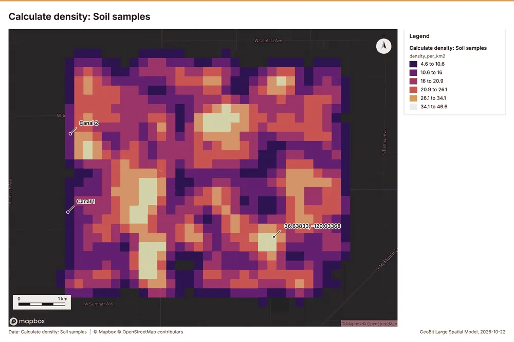
Why it was run on this data. 600 points in Soil samples: a density surface shows where they concentrate 42.
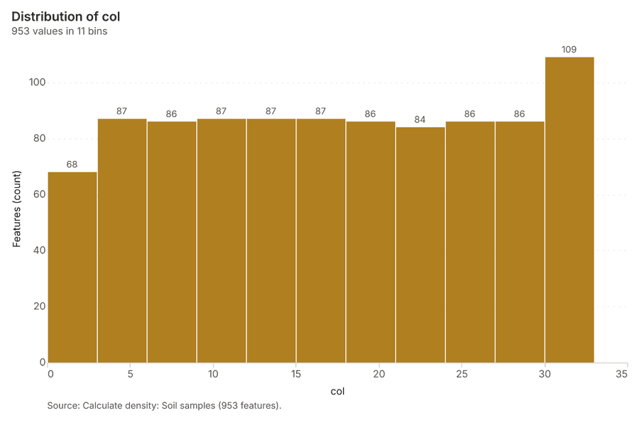
What it found. Calculate density on Soil samples: Calculate density: 1 layer saved: Calculate density: Soil samples (953 features) 2043. It reported result, count 953; result, elapsed ms 30; result, bandwidth m 500; result, cell size m 200; result, excluded null 0; result, max density per km2 46.63 43.
| Result | Value |
|---|---|
| result, count | 953 |
| result, elapsed ms | 30 |
| result, bandwidth m | 500 |
| result, cell size m | 200 |
| result, excluded null | 0 |
| result, max density per km2 | 46.63 |
| billing, cost | 0.062 |
| billing, list price | 0.062 |
| billing, upstream cost | 0 |
Findings
- Evidenced: Calculate density on Soil samples: Calculate density: 1 layer saved: Calculate density: Soil samples (953 features) 2043.
- Evidenced: It reported result, count 953; result, elapsed ms 30; result, bandwidth m 500; result, cell size m 200; result, excluded null 0; result, max density per km2 46.63 43.
Tool gp_calculate_density; parameters {"kernel": "quartic", "project": "c0ff746c-cbbb-48c5-a026-444453a7b463", "features": {"layer": "Soil samples (caf67b23)"}, "bandwidth_m": 500.0, "cell_size_m": 200.0}
Find point clusters
What this analysis is. Find point clusters: Density-based clusters (DBSCAN, HDBSCAN or OPTICS, optionally space-time) with hulls and noise 44. In ArcGIS it is Find Point Clusters or Density-based Clustering; in QGIS, native:dbscanclustering or native:stdbscanclustering 44.
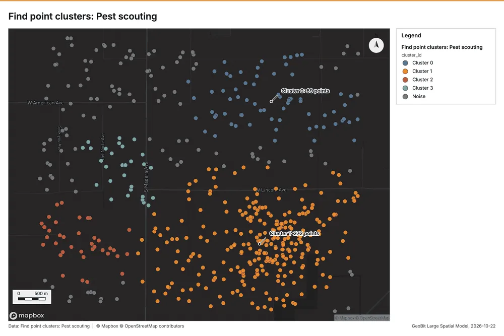
Why it was run on this data. DBSCAN finds dense groups of Pest scouting and separates noise 45.
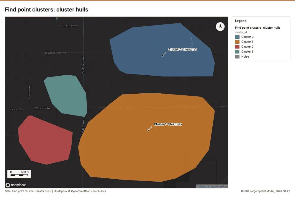
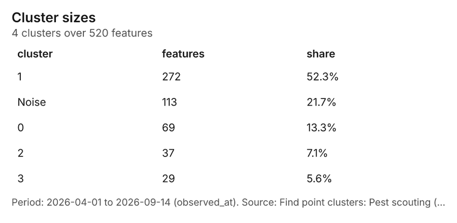
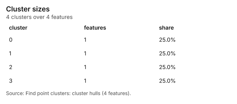
What it found. Find point clusters on Pest scouting: Find point clusters: 2 layers saved: Find point clusters: Pest scouting (520 features); Find point clusters: cluster hulls (4 features) 1246. It reported result, count 520; result, noise 113; result, distance m 500; result, elapsed ms 13; result, min points 13; billing, cost 0.0604 46.
| Result | Value |
|---|---|
| result, count | 520 |
| result, noise | 113 |
| result, distance m | 500 |
| result, elapsed ms | 13 |
| result, min points | 13 |
| billing, cost | 0.0604 |
| billing, list price | 0.0604 |
| billing, upstream cost | 0 |
Findings
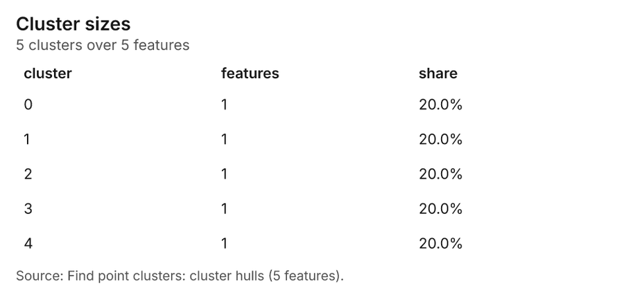
- Evidenced: Find point clusters on Pest scouting: Find point clusters: 2 layers saved: Find point clusters: Pest scouting (520 features); Find point clusters: cluster hulls (4 features) 1246.
- Evidenced: It reported result, count 520; result, noise 113; result, distance m 500; result, elapsed ms 13; result, min points 13; billing, cost 0.0604 46.
Tool gp_find_point_clusters; parameters {"method": "dbscan", "project": "c0ff746c-cbbb-48c5-a026-444453a7b463", "features": {"layer": "Pest scouting (815c2b2c)"}, "distance_m": 500.0, "min_points": 13}
Find point clusters
What this analysis is. Find point clusters: Density-based clusters (DBSCAN, HDBSCAN or OPTICS, optionally space-time) with hulls and noise 44. In ArcGIS it is Find Point Clusters or Density-based Clustering; in QGIS, native:dbscanclustering or native:stdbscanclustering 44.
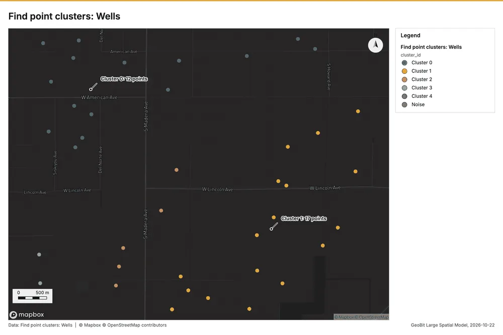
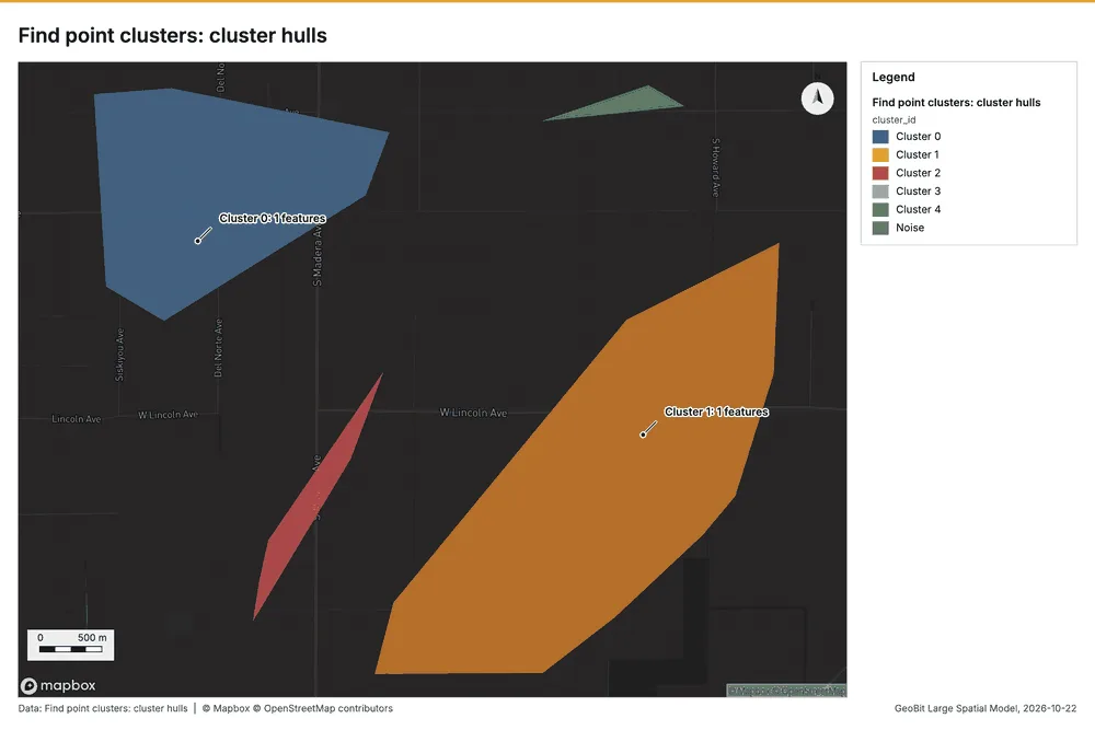
Why it was run on this data. DBSCAN finds dense groups of Wells and separates noise 47.
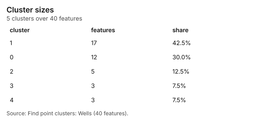
What it found. Find point clusters on Wells: Find point clusters: 2 layers saved: Find point clusters: Wells (40 features); Find point clusters: cluster hulls (5 features) 1448. It reported result, count 40; result, noise 0; result, distance m 1,000; result, elapsed ms 3; result, min points 3; billing, cost 0.0508 48.
| Result | Value |
|---|---|
| result, count | 40 |
| result, noise | 0 |
| result, distance m | 1,000 |
| result, elapsed ms | 3 |
| result, min points | 3 |
| billing, cost | 0.0508 |
| billing, list price | 0.0508 |
| billing, upstream cost | 0 |
Findings
- Evidenced: Find point clusters on Wells: Find point clusters: 2 layers saved: Find point clusters: Wells (40 features); Find point clusters: cluster hulls (5 features) 1448.
- Evidenced: It reported result, count 40; result, noise 0; result, distance m 1,000; result, elapsed ms 3; result, min points 3; billing, cost 0.0508 48.
Tool gp_find_point_clusters; parameters {"method": "dbscan", "project": "c0ff746c-cbbb-48c5-a026-444453a7b463", "features": {"layer": "Wells (15d08948)"}, "distance_m": 1000.0, "min_points": 3}
Find point clusters
What this analysis is. Find point clusters: Density-based clusters (DBSCAN, HDBSCAN or OPTICS, optionally space-time) with hulls and noise 44. In ArcGIS it is Find Point Clusters or Density-based Clustering; in QGIS, native:dbscanclustering or native:stdbscanclustering 44.
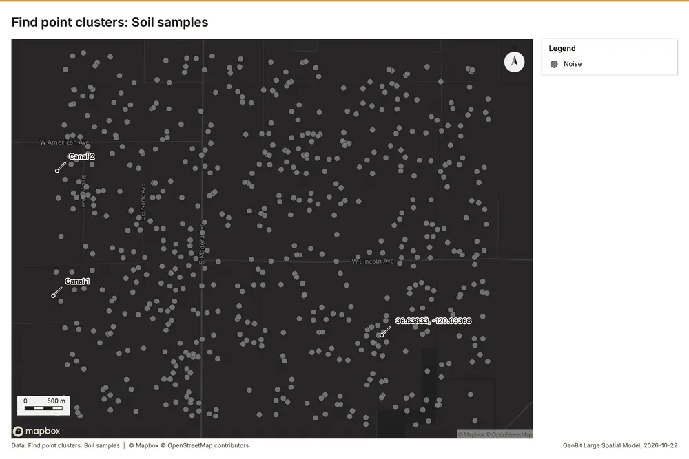
Why it was run on this data. DBSCAN finds dense groups of Soil samples and separates noise 49.
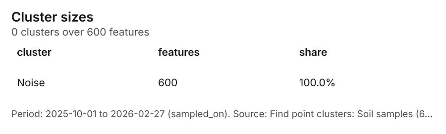
What it found. Find point clusters on Soil samples: Find point clusters: 1 layer saved: Find point clusters: Soil samples (600 features) 2050. It reported result, count 600; result, noise 600; result, distance m 200; result, elapsed ms 9; result, min points 15; billing, cost 0.062 50.
| Result | Value |
|---|---|
| result, count | 600 |
| result, noise | 600 |
| result, distance m | 200 |
| result, elapsed ms | 9 |
| result, min points | 15 |
| billing, cost | 0.062 |
| billing, list price | 0.062 |
| billing, upstream cost | 0 |
Findings
- Evidenced: Find point clusters on Soil samples: Find point clusters: 1 layer saved: Find point clusters: Soil samples (600 features) 2050.
- Evidenced: It reported result, count 600; result, noise 600; result, distance m 200; result, elapsed ms 9; result, min points 15; billing, cost 0.062 50.
Tool gp_find_point_clusters; parameters {"method": "dbscan", "project": "c0ff746c-cbbb-48c5-a026-444453a7b463", "features": {"layer": "Soil samples (caf67b23)"}, "distance_m": 200.0, "min_points": 15}
Zonal statistics
What this analysis is. Zonal statistics: count/min/max/mean/std/sum/median/majority per polygon as a table and as GeoJSON 51. In ArcGIS it is Zonal Statistics as Table (polygons) 51.
Why it was run on this data. Statistics of Satellite scene 2026-04-15 inside each feature of Fields 52.
What it found. The analysis used the Zonal statistics tool, specifically rs_zonal_statistics, at step 0 53. This process resulted in 60 row(s) of data 53. Furthermore, the zonal statistics encompassed a total of 60 zones 53.
Findings
Tool rs_zonal_statistics; parameters {"stats": ["mean", "min", "max", "std"], "zones": "Fields (a196eb79)", "raster_id": "Satellite scene 2026-04-15 (6c1f22ed)"}
Zonal statistics
What this analysis is. Zonal statistics: count/min/max/mean/std/sum/median/majority per polygon as a table and as GeoJSON 51. In ArcGIS it is Zonal Statistics as Table (polygons) 51.
Why it was run on this data. Statistics of Satellite scene 2026-04-15 inside each feature of Fields 52.
What it found. The analysis utilized the Zonal statistics tool, specifically rs_zonal_statistics 54. The results indicate an output containing 60 rows 54. Furthermore, the process calculated statistics across 60 distinct zones 54.
Findings
Tool rs_zonal_statistics; parameters {"stats": ["mean", "min", "max", "std"], "zones": "Fields (a196eb79)", "raster_id": "Satellite scene 2026-08-15 (34efa462)"}
Maps and charts
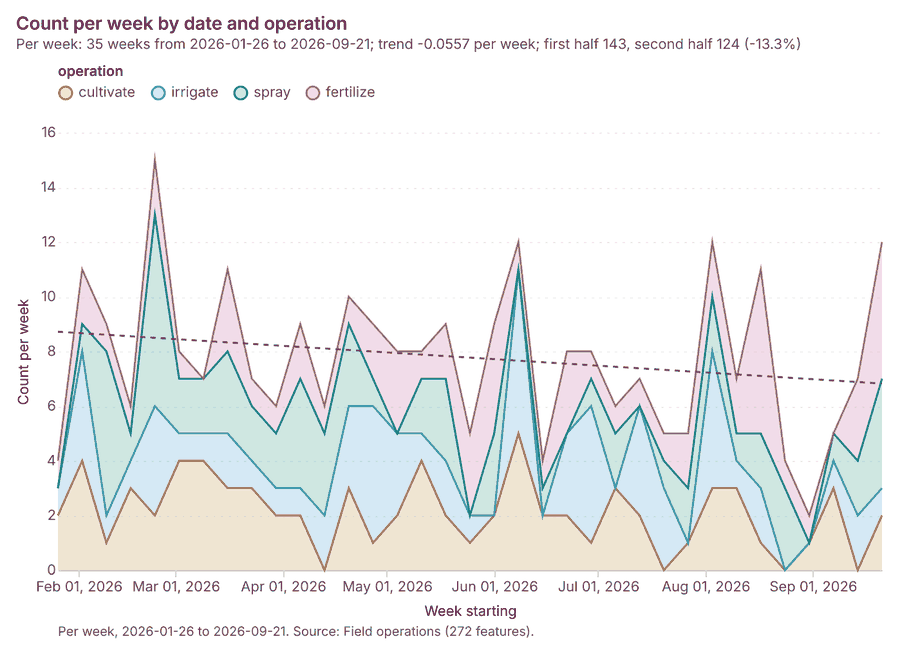
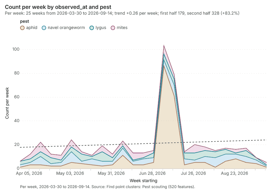
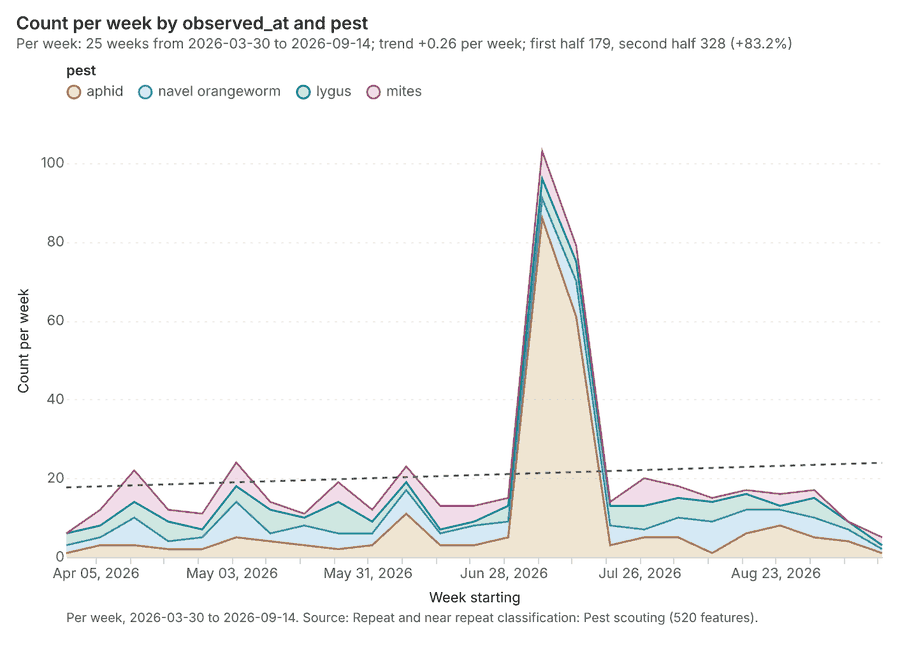
The run also made 22 map image(s) 55565758596061626364656667686970717273747576 and 23 chart(s) 7778798081828384858687888990919293949596979899.
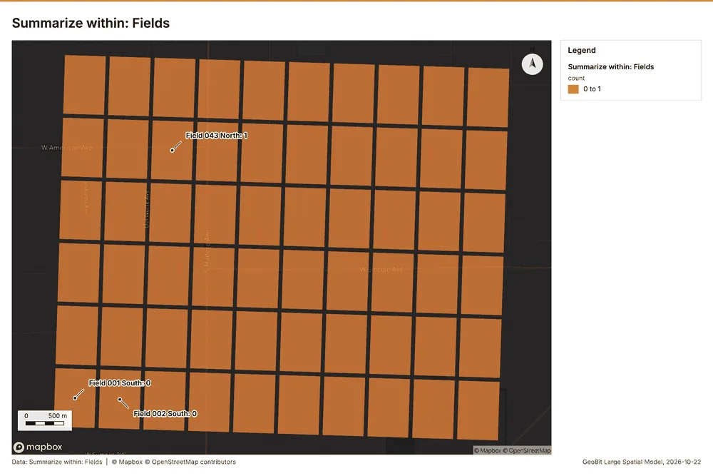
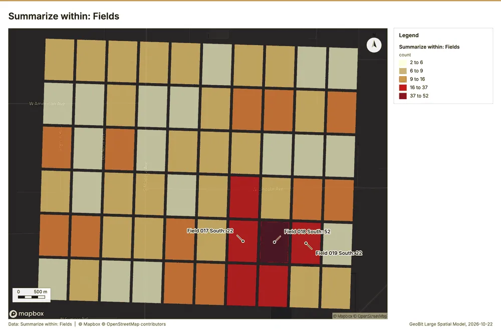
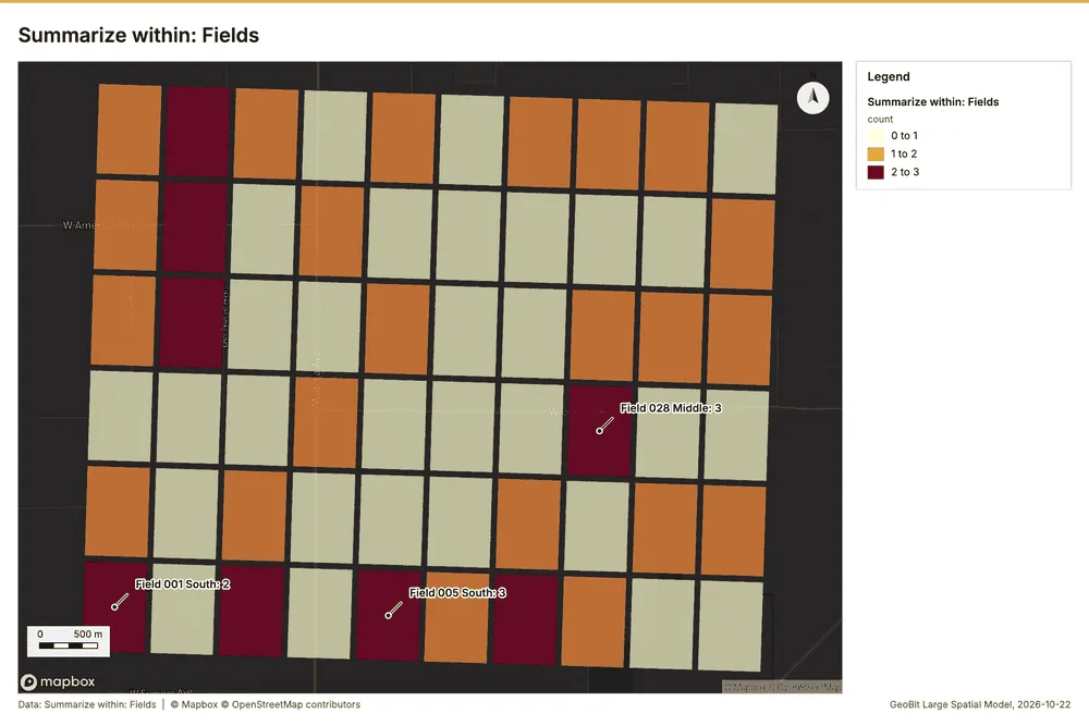
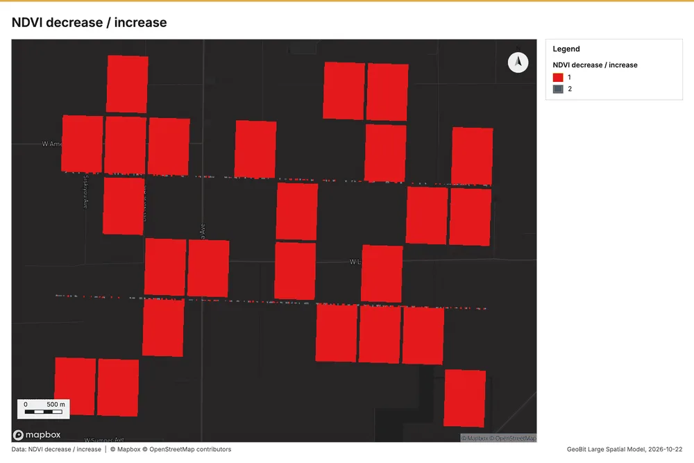
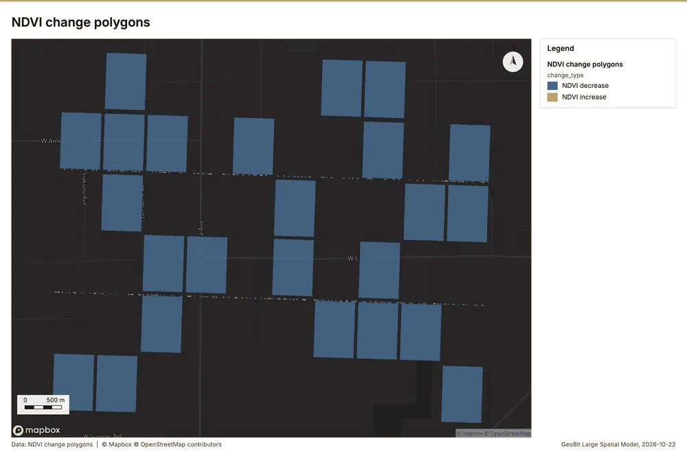
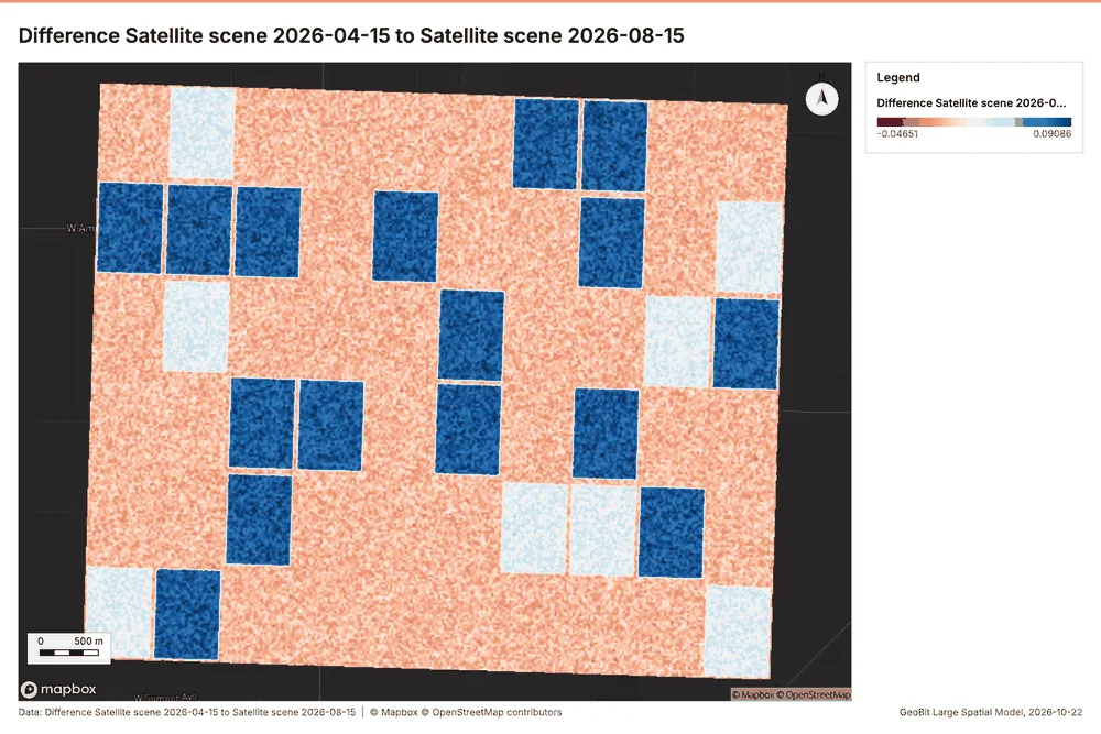
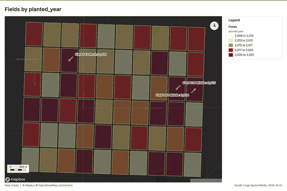
What the map shows. This map illustrates the concentration of "Fields" across the area, 57
Inferred: read from the image by gemma4:e4b, not evidence.
Changes since the last run
This is the first report of this project.
Sources
- 1Rendering: Chart: Timeline: events per quarter by dataset. 92 rows id 210bf478-e864-4742-9c56-7c7e371b620c
- 2Dataset: Soil samples. vector, 600 rows id f4ae2248-8882-412c-b6a9-09b418581a65
- 3Dataset: Pest scouting. vector, 520 rows id 63eec720-9e01-4dce-9c81-975e42e92d0b
- 4Dataset: Yields by season. table, 300 rows id a530983b-a4cf-4197-96b4-ac4ee482921b
- 5Dataset: Field operations. table, 272 rows id a8bf3d14-5f38-4346-878a-d28bc636b06e
- 6Catalog: Summarize within (operation catalog, gp_summarize_within). Count and aggregate the features inside each polygon (or bin), proportionally for lines and polygons. ArcGIS: Summarize Within, Aggregate Points. QGIS: native:countpointsinpolygon, native:sumlinelengths. id gp_summarize_within
- 7Plan: Weather stations per feature of Fields (the Start plan's candidate c_454a5cc5eea8). Count Weather stations inside each feature of Fields; the counts map as a choropleth (natural breaks, sequential colors). id ae3647a3-d230-4a37-b0e8-19aa34415db3:c_454a5cc5eea8
- 8Tool result: gp_summarize_within, step 0. Summarize within: 1 layer saved: Summarize within: Fields (60 features). id dccd77e6-8290-42cb-9255-e52125568f63:0
- 9Layer: Weather stations. 3 features id 7a8242c6-adef-4d23-9e5b-df9ccaca27ad
- 10Layer: Fields. 60 features id a196eb79-1c58-44ab-9608-3f8de23cc587
- 11Tool result: gp_summarize_within, step 1. Summarize within: 1 layer saved: Summarize within: Fields (60 features). id dccd77e6-8290-42cb-9255-e52125568f63:1
- 12Layer: Pest scouting. 520 features id 815c2b2c-fc4f-4927-8f05-1744f43ca273
- 13Tool result: gp_summarize_within, step 2. Summarize within: 1 layer saved: Summarize within: Fields (60 features). id dccd77e6-8290-42cb-9255-e52125568f63:2
- 14Layer: Wells. 40 features id 15d08948-7e45-4cf2-ad71-6bb21299a25d
- 15Catalog: Emerging hot spots (operation catalog, gp_space_time_hot_spots). Where hot spots are new, consecutive, intensifying, persistent, diminishing, sporadic, oscillating or historical over time. ArcGIS: Emerging Hot Spot Analysis, Create Space Time Cube. id gp_space_time_hot_spots
- 16Plan: Space time hot spots of Pest scouting (the Start plan's candidate c_45dd616af1e5). Pest scouting carry dates in 'observed_at': emerging hot spot analysis finds new, intensifying and fading hot spots per week. id ae3647a3-d230-4a37-b0e8-19aa34415db3:c_45dd616af1e5
- 17Tool result: gp_space_time_hot_spots, step 0. Emerging hot spots: 1 layer saved: Emerging hot spots: Pest scouting (48 features). id 4244d4f5-f923-4458-9154-022dacee4c61:0
- 18Plan: Space time hot spots of Soil samples (the Start plan's candidate c_850c0bb45f60). Soil samples carry dates in 'sampled_on': emerging hot spot analysis finds new, intensifying and fading hot spots per week. id ae3647a3-d230-4a37-b0e8-19aa34415db3:c_850c0bb45f60
- 19Tool result: gp_space_time_hot_spots, step 1. Emerging hot spots: 1 layer saved: Emerging hot spots: Soil samples (51 features). id 4244d4f5-f923-4458-9154-022dacee4c61:1
- 20Layer: Soil samples. 600 features id caf67b23-0043-4bf5-8531-43267ce2ed9f
- 21Catalog: Repeat and near repeat classification (operation catalog, gp_near_repeat). Classify incidents as originators, repeats (same place) or near repeats within a distance and time window, with a Knox test table. ArcGIS: Repeat and Near Repeat Classification, Near Repeat Calculator. id gp_near_repeat
- 22Plan: Near repeat of Pest scouting (the Start plan's candidate c_a26d0b1eb35d). Near repeat analysis tests whether Pest scouting close in space also follow each other within 17 days. id ae3647a3-d230-4a37-b0e8-19aa34415db3:c_a26d0b1eb35d
- 23Tool result: gp_near_repeat, step 2. Repeat and near repeat classification: 1 layer saved: Repeat and near repeat classification: Pest scouting (520 features). id 4244d4f5-f923-4458-9154-022dacee4c61:2
- 24Catalog: Spectral index change (analysis catalog, im_index_change). Change of a spectral index (NDVI, NDWI, NDBI, NBR ...) or a band expression between two images: before, after and difference rasters, decrease / increase classes beyond the threshold with polygons and areas; NBR also gives dNBR with burn severity classes. id im_index_change
- 25Plan: Index change of Satellite scene 2026-04-15 and Satellite scene 2026-08-15 (the Start plan's candidate c_09e02b8174f1). Index change between Satellite scene 2026-04-15 (2026-04-15) and Satellite scene 2026-08-15 (2026-08-15): the changed area, with the changed places as polygons. id ae3647a3-d230-4a37-b0e8-19aa34415db3:c_09e02b8174f1
- 26Tool result: im_index_change, step 0. Spectral index change: created NDVI change Satellite scene 2026-04-15 to Satellite scene 2026-08-15 (300 x 250 cells, 20.00 m). plus 1 more raster layer(s). and layer NDVI change polygons with 175 feature(s). mean before 0.7068; mean after 0.5038; mean difference -0.203; decrease ha 1,053; increase id aa0bd809-0fe9-498d-b9f1-719c7c0e70f8:0
- 27Catalog: Compute change raster (analysis catalog, im_compute_change_raster). Pixel value or spectral change between two co-registered images: difference, relative difference, absolute difference, log ratio (radar, dB), Euclidean spectral distance, spectral angle (radians) or the band with most change. Clouds and shadows are masked when the images have id im_compute_change_raster
- 28Plan: Compute change raster of Satellite scene 2026-04-15 and Satellite scene 2026-08-15 (the Start plan's candidate c_c88ddec02454). A change raster between Satellite scene 2026-04-15 (2026-04-15) and Satellite scene 2026-08-15 (2026-08-15): where and how much the pixels changed. id ae3647a3-d230-4a37-b0e8-19aa34415db3:c_c88ddec02454
- 29Tool result: im_compute_change_raster, step 1. Compute change raster: created Difference Satellite scene 2026-04-15 to Satellite scene 2026-08-15 (300 x 250 cells, 20.00 m). mean 0.02217; std 0.03434; min -0.037; max 0.116; masked pixels 0. id aa0bd809-0fe9-498d-b9f1-719c7c0e70f8:1
- 30Catalog: Hot spot analysis (operation catalog, gp_hot_spots). Getis-Ord Gi* hot and cold spots with z-scores, p-values and confidence bins. ArcGIS: Find Hot Spots, Hot Spot Analysis (Getis-Ord Gi*). QGIS: qgis:hotspot (plugin). id gp_hot_spots
- 31Plan: Hot spots of Pest scouting (the Start plan's candidate c_e6241d85c30d). 520 points: Getis-Ord Gi* tests whether the concentrations in Pest scouting are statistically significant. id ae3647a3-d230-4a37-b0e8-19aa34415db3:c_e6241d85c30d
- 32Tool result: gp_hot_spots, step 0. Hot spot analysis: 1 layer saved: Hot spot analysis: Pest scouting (134 features). id abe0cc5c-b82d-4992-9626-cf301845c602:0
- 33Plan: Hot spots of Wells (the Start plan's candidate c_5a29d39e7d24). 40 points: Getis-Ord Gi* tests whether the concentrations in Wells are statistically significant. id ae3647a3-d230-4a37-b0e8-19aa34415db3:c_5a29d39e7d24
- 34Tool result: gp_hot_spots, step 1. Hot spot analysis: 1 layer saved: Hot spot analysis: Wells (13 features). id abe0cc5c-b82d-4992-9626-cf301845c602:1
- 35Plan: Hot spots of Soil samples (the Start plan's candidate c_236d56d345ee). 600 points: Getis-Ord Gi* tests whether the concentrations in Soil samples are statistically significant. id ae3647a3-d230-4a37-b0e8-19aa34415db3:c_236d56d345ee
- 36Tool result: gp_hot_spots, step 2. Hot spot analysis: 1 layer saved: Hot spot analysis: Soil samples (139 features). id abe0cc5c-b82d-4992-9626-cf301845c602:2
- 37Catalog: Calculate density (operation catalog, gp_calculate_density). Kernel density per square kilometer on a grid. ArcGIS: Calculate Density, Kernel Density. QGIS: native:heatmapkerneldensityestimation. id gp_calculate_density
- 38Plan: Kernel density of Pest scouting (the Start plan's candidate c_a69023aa1d48). 520 points in Pest scouting: a density surface shows where they concentrate. id ae3647a3-d230-4a37-b0e8-19aa34415db3:c_a69023aa1d48
- 39Tool result: gp_calculate_density, step 0. Calculate density: 1 layer saved: Calculate density: Pest scouting (937 features). id 0aef980e-7aff-47d5-becc-3abd115d0df6:0
- 40Plan: Kernel density of Wells (the Start plan's candidate c_f362031aa57c). 40 points in Wells: a density surface shows where they concentrate. id ae3647a3-d230-4a37-b0e8-19aa34415db3:c_f362031aa57c
- 41Tool result: gp_calculate_density, step 1. Calculate density: 1 layer saved: Calculate density: Wells (75 features). id 0aef980e-7aff-47d5-becc-3abd115d0df6:1
- 42Plan: Kernel density of Soil samples (the Start plan's candidate c_031ecade8328). 600 points in Soil samples: a density surface shows where they concentrate. id ae3647a3-d230-4a37-b0e8-19aa34415db3:c_031ecade8328
- 43Tool result: gp_calculate_density, step 2. Calculate density: 1 layer saved: Calculate density: Soil samples (953 features). id 0aef980e-7aff-47d5-becc-3abd115d0df6:2
- 44Catalog: Find point clusters (operation catalog, gp_find_point_clusters). Density-based clusters (DBSCAN, HDBSCAN or OPTICS, optionally space-time) with hulls and noise. ArcGIS: Find Point Clusters, Density-based Clustering. QGIS: native:dbscanclustering, native:stdbscanclustering. id gp_find_point_clusters
- 45Plan: Cluster points of Pest scouting (the Start plan's candidate c_d5b8ebbc13e3). DBSCAN finds dense groups of Pest scouting and separates noise. id ae3647a3-d230-4a37-b0e8-19aa34415db3:c_d5b8ebbc13e3
- 46Tool result: gp_find_point_clusters, step 0. Find point clusters: 2 layers saved: Find point clusters: Pest scouting (520 features); Find point clusters: cluster hulls (4 features). id d3e49c76-baed-436b-aed4-42467a2d8691:0
- 47Plan: Cluster points of Wells (the Start plan's candidate c_cb6793249bdf). DBSCAN finds dense groups of Wells and separates noise. id ae3647a3-d230-4a37-b0e8-19aa34415db3:c_cb6793249bdf
- 48Tool result: gp_find_point_clusters, step 1. Find point clusters: 2 layers saved: Find point clusters: Wells (40 features); Find point clusters: cluster hulls (5 features). id d3e49c76-baed-436b-aed4-42467a2d8691:1
- 49Plan: Cluster points of Soil samples (the Start plan's candidate c_c62ca5d55d3c). DBSCAN finds dense groups of Soil samples and separates noise. id ae3647a3-d230-4a37-b0e8-19aa34415db3:c_c62ca5d55d3c
- 50Tool result: gp_find_point_clusters, step 2. Find point clusters: 1 layer saved: Find point clusters: Soil samples (600 features). id d3e49c76-baed-436b-aed4-42467a2d8691:2
- 51Catalog: Zonal statistics (analysis catalog, rs_zonal_statistics). count/min/max/mean/std/sum/median/majority per polygon as a table and as GeoJSON. ArcGIS: Zonal Statistics as Table (polygons). id rs_zonal_statistics
- 52Plan: Zonal statistics of Satellite scene 2026-04-15 and Fields (the Start plan's candidate c_e314d28606e4). Statistics of Satellite scene 2026-04-15 inside each feature of Fields. id ae3647a3-d230-4a37-b0e8-19aa34415db3:c_e314d28606e4
- 53Tool result: rs_zonal_statistics, step 0. Zonal statistics: 60 row(s). zones 60. id 65e47d44-0efb-439a-97dd-b6f970b5def8:0
- 54Tool result: rs_zonal_statistics, step 1. Zonal statistics: 60 row(s). zones 60. id 65e47d44-0efb-439a-97dd-b6f970b5def8:1
- 55Rendering: Map: Summarize within: Fields id 7230104f-7ded-41b5-8137-03d3472c4fda
- 56Rendering: Map: Summarize within: Fields id 8653af7e-4e73-4408-a171-1f6950196dca
- 57Rendering: Map: Summarize within: Fields id 7cd707d4-3613-4819-8d43-7e3c43279eac
- 58Rendering: Map: Emerging hot spots: Pest scouting id b78dba51-33f9-4ea8-835a-48251bebd889
- 59Rendering: Map: Emerging hot spots: Soil samples id 391b8c8e-89d7-4099-a7bb-e45b7ee88e6b
- 60Rendering: Map: Repeat and near repeat classification: Pest scouting id 90157d45-c4a6-4d1d-9dcf-b704c93e0eb5
- 61Rendering: Map: NDVI change Satellite scene 2026-04-15 to Satellite scene 2026-08-15 id 0de86fc2-8ff8-4ce7-b077-43a5ab4bb376
- 62Rendering: Map: NDVI decrease / increase id e74e322f-5c79-4f18-a2f6-d502e8b31d86
- 63Rendering: Map: NDVI change polygons id 89e60139-e1e3-409e-8bc0-bcf9c32a5e30
- 64Rendering: Map: Difference Satellite scene 2026-04-15 to Satellite scene 2026-08-15 id df6ad400-4033-420c-8150-f286d0d0ce02
- 65Rendering: Map: Fields by planted_year id b7bcce2d-b7d0-4b90-bed2-1e960095b8f5
- 66Rendering: Map: Hot spot analysis: Pest scouting id 3a23b5af-27f8-49c6-bf66-fa49b20a08aa
- 67Rendering: Map: Hot spot analysis: Wells id cd3c7db8-cfb5-4aed-809a-15a9c2e1ee04
- 68Rendering: Map: Hot spot analysis: Soil samples id 94b47520-81ad-4a35-9ed1-2ed221c66501
- 69Rendering: Map: Calculate density: Pest scouting id bf1a8ba7-ca53-469d-b24c-54ae7dbb680b
- 70Rendering: Map: Calculate density: Wells id fa642946-bff5-47a9-a9cd-c67b1f2f7bfe
- 71Rendering: Map: Calculate density: Soil samples id 8413c226-61fc-4fdd-92b1-023ff3edb997
- 72Rendering: Map: Find point clusters: Pest scouting id 51fe83ea-2c87-4a9e-8844-7feb42f6f11a
- 73Rendering: Map: Find point clusters: cluster hulls id e7e8fe55-e846-4d44-a326-06cac7e2cfca
- 74Rendering: Map: Find point clusters: Wells id fed095c7-3edc-4fd2-a373-d17fc6251739
- 75Rendering: Map: Find point clusters: cluster hulls id 400e2024-a606-405d-8c29-65b08ce86104
- 76Rendering: Map: Find point clusters: Soil samples id 37d0f2ff-28af-4ea5-88ad-7955526003bf
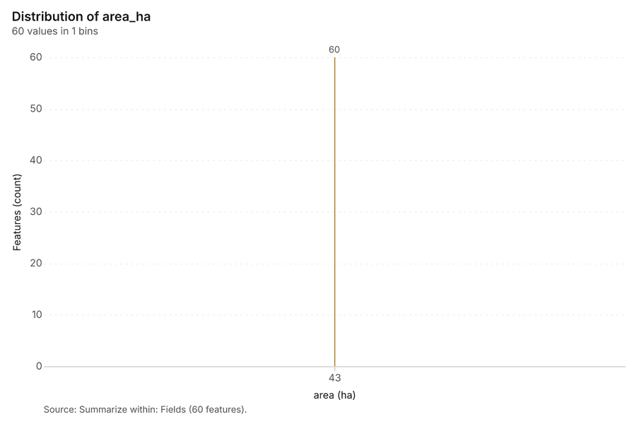
- 77Rendering: Chart: Fields over time (planted_year). 1 rows id 4fae63f6-4165-4c37-9583-b5e8b7fbe000
- 78Rendering: Chart: Field operations over time (date). 140 rows id 2b4ce56e-b8f2-4990-87a1-8e81d44ab30b
- 79Rendering: Chart: Summarize within: Fields. 1 rows id f44f0c04-6401-435e-908e-61b78a5cedb0
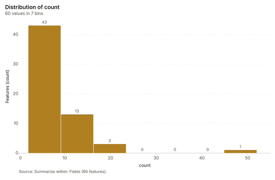
- 80Rendering: Chart: Summarize within: Fields. 7 rows id e36c7df7-7eb0-4113-a898-84173c1635a7
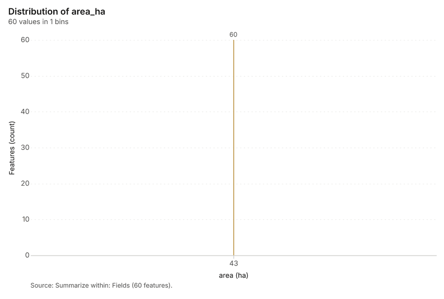
- 81Rendering: Chart: Summarize within: Fields. 1 rows id b56c5a2b-ea58-4c97-871a-e80878d78549
- 82Rendering: Chart: Emerging hot spots: Pest scouting. 7 rows id 314c5791-c320-418e-8128-46033cad4c68
- 83Rendering: Chart: Emerging hot spots: Soil samples. 7 rows id 212eb454-b769-41a6-8a5f-e897a360eff2
- 84Rendering: Chart: Repeat and near repeat classification: Pest scouting. 100 rows id 4ec337e3-0fad-4735-a5cd-35ba6454f64c
- 85Rendering: Chart: NDVI change polygons. 9 rows id b6caeb8f-73bd-4c12-bb71-811ad9d4f4fc
- 86Rendering: Chart: Hot spot analysis: Pest scouting. 11 rows id 11c79607-7ed1-452c-ab6e-436e1580c59b
- 87Rendering: Chart: Hot spot analysis: Wells. 7 rows id 5e81ab47-dc6c-4c0b-bf73-cb9a953888c8
- 88Rendering: Chart: Hot spot analysis: Soil samples. 10 rows id aa8f7bb7-d4a0-4160-acf0-4c3df1175537
- 89Rendering: Chart: Calculate density: Pest scouting. 11 rows id cb76c785-37e5-43e8-8f0d-40da98f49b28
- 90Rendering: Chart: Calculate density: Wells. 8 rows id 542ea61d-ff29-475d-b5fa-ebe52baa7deb
- 91Rendering: Chart: Calculate density: Soil samples. 11 rows id 07136eeb-2846-4054-ab99-30695bfabe15
- 92Rendering: Chart: Find point clusters: Pest scouting. 5 rows id 281d1a9c-7ff6-4172-a7c6-6af005d6f6bb
- 93Rendering: Chart: Find point clusters: cluster hulls. 4 rows id 133c6e8d-eb2d-492b-8bbb-1a76f6947626
- 94Rendering: Chart: Find point clusters: Wells. 5 rows id 647d827f-dbff-458c-b5c6-646ed6c20169
- 95Rendering: Chart: Find point clusters: cluster hulls. 5 rows id ca4b1c22-b048-4fd3-8fe4-a0d9efa5b4ae
- 96Rendering: Chart: Find point clusters: Soil samples. 1 rows id fec77e96-06d0-41b0-93d3-a8270db698ce
- 97Rendering: Chart: Find point clusters: Soil samples over time. 22 rows id 4fc7d651-51f3-4c40-90d5-b49a93b06ea2
- 98Rendering: Chart: Find point clusters: Pest scouting over time. 100 rows id 9aedbf91-7578-44d6-98ab-cb2d3aa2bc15
- 99Rendering: Chart: Repeat and near repeat classification: Pest scouting over time. 100 rows id 32669449-e850-4080-86e2-4007127d571f
- 100Dataset: Fields. vector, 60 rows id ae5ec258-e5f4-4d17-bdc8-60502e957eff
- 101Dataset: Satellite scene 2026-04-15. raster, ? rows id afcb6073-f5d0-4e9b-9733-f8ff25683e32
- 102Dataset: Satellite scene 2026-08-15. raster, ? rows id e159db17-63d9-49cf-89e5-b0ae9c8b48a2
- 103Dataset: Irrigation canals. vector, 5 rows id 97634f60-fee7-4f4e-a64e-637edfb86b11
- 104Dataset: Wells. vector, 40 rows id 74fc7b42-f33b-42ca-8b5d-9cfcb97c141a
- 105Dataset: Weather stations. vector, 3 rows id 0f5f59b7-502a-40bb-b75d-bdadd47f3080
- 106Dataset: Agronomist season notes. document, ? rows id d84db76e-6efd-462b-9106-b94192b7b788
- 107Record: Sample: Agriculture, Fresno County id c0ff746c-cbbb-48c5-a026-444453a7b463
- 108Layer: Summarize within: Fields. 60 features id b2fdbfbb-e5aa-42e7-94a1-89a27706bffe
- 109Layer: Summarize within: Fields. 60 features id 4f0023ee-b3ec-488f-bf30-f0fc9b0f5b3a
- 110Layer: Summarize within: Fields. 60 features id 951c1d69-082b-442b-a64e-e85bf3484a2f
- 111Layer: Emerging hot spots: Pest scouting. 48 features id 0be5bf67-1fa9-4a8c-83c8-e34bc93079d1
- 112Layer: Emerging hot spots: Soil samples. 51 features id 2a629716-c8ab-4b63-9c37-e87b9441d065
- 113Layer: Repeat and near repeat classification: Pest scouting. 520 features id fe782344-23a8-476a-b62d-d355ef2335ff
- 114Layer: NDVI change Satellite scene 2026-04-15 to Satellite scene 2026-08-15. 0 features id 8e44c499-3d6d-40a2-bf98-2aadc140cd8a
- 115Layer: NDVI decrease / increase. 0 features id bb4c7791-d581-4575-8cb4-3ef1435080f6
- 116Layer: NDVI change polygons. 175 features id f16ca8cc-e568-476b-891d-77e47b995583
- 117Layer: Difference Satellite scene 2026-04-15 to Satellite scene 2026-08-15. 0 features id a67372cb-7b7e-4c71-947c-5b97fba5d52f
- 118Layer: Hot spot analysis: Pest scouting. 134 features id 9e178787-e1af-447d-b9a8-b00743fc24e6
- 119Layer: Hot spot analysis: Wells. 13 features id d441f28d-a4a4-41b6-ae29-45dd731e936a
- 120Layer: Hot spot analysis: Soil samples. 139 features id 8e554e35-3a16-4452-9c1b-514be82182a7
- 121Layer: Calculate density: Pest scouting. 937 features id c70c03ec-c02f-4e66-b411-9818647d6aeb
- 122Layer: Calculate density: Wells. 75 features id 5b6288ae-67ae-41cd-84c7-b081bfc8198d
- 123Layer: Calculate density: Soil samples. 953 features id 1b537a1d-851e-429a-a0a3-2796431cad1c
- 124Layer: Find point clusters: Pest scouting. 520 features id 531e30e6-075f-4448-8903-ceb10bcec608
- 125Layer: Find point clusters: cluster hulls. 4 features id 3290f356-6d63-4379-ad57-5da11d5df04b
- 126Layer: Find point clusters: Wells. 40 features id 4497616c-038d-4f7d-bfd7-4a1fba479ca8
- 127Layer: Find point clusters: cluster hulls. 5 features id 973c4eb5-10d8-4c78-81b4-8d4b2dce4966
- 128Layer: Find point clusters: Soil samples. 600 features id a1768046-65e4-431b-b327-112b2874c867
Appendix: the data behind the chartsShow
Figure 1. Timeline: events per quarter by dataset 1
| period | series | value |
|---|---|---|
| 2021-01-01 | Soil samples | 0 |
| 2021-01-01 | Pest scouting | 0 |
| 2021-01-01 | Yields by season | 60 |
| 2021-01-01 | Field operations | 0 |
| 2021-04-01 | Soil samples | 0 |
| 2021-04-01 | Pest scouting | 0 |
| 2021-04-01 | Yields by season | 0 |
| 2021-04-01 | Field operations | 0 |
| 2021-07-01 | Soil samples | 0 |
| 2021-07-01 | Pest scouting | 0 |
| 2021-07-01 | Yields by season | 0 |
| 2021-07-01 | Field operations | 0 |
| 2021-10-01 | Soil samples | 0 |
| 2021-10-01 | Pest scouting | 0 |
| 2021-10-01 | Yields by season | 0 |
| 2021-10-01 | Field operations | 0 |
| 2022-01-01 | Soil samples | 0 |
| 2022-01-01 | Pest scouting | 0 |
| 2022-01-01 | Yields by season | 60 |
| 2022-01-01 | Field operations | 0 |
| 2022-04-01 | Soil samples | 0 |
| 2022-04-01 | Pest scouting | 0 |
| 2022-04-01 | Yields by season | 0 |
| 2022-04-01 | Field operations | 0 |
| 2022-07-01 | Soil samples | 0 |
| 2022-07-01 | Pest scouting | 0 |
| 2022-07-01 | Yields by season | 0 |
| 2022-07-01 | Field operations | 0 |
| 2022-10-01 | Soil samples | 0 |
| 2022-10-01 | Pest scouting | 0 |
| 2022-10-01 | Yields by season | 0 |
| 2022-10-01 | Field operations | 0 |
| 2023-01-01 | Soil samples | 0 |
| 2023-01-01 | Pest scouting | 0 |
| 2023-01-01 | Yields by season | 60 |
| 2023-01-01 | Field operations | 0 |
| 2023-04-01 | Soil samples | 0 |
| 2023-04-01 | Pest scouting | 0 |
| 2023-04-01 | Yields by season | 0 |
| 2023-04-01 | Field operations | 0 |
| 2023-07-01 | Soil samples | 0 |
| 2023-07-01 | Pest scouting | 0 |
| 2023-07-01 | Yields by season | 0 |
| 2023-07-01 | Field operations | 0 |
| 2023-10-01 | Soil samples | 0 |
| 2023-10-01 | Pest scouting | 0 |
| 2023-10-01 | Yields by season | 0 |
| 2023-10-01 | Field operations | 0 |
| 2024-01-01 | Soil samples | 0 |
| 2024-01-01 | Pest scouting | 0 |
| 2024-01-01 | Yields by season | 60 |
| 2024-01-01 | Field operations | 0 |
| 2024-04-01 | Soil samples | 0 |
| 2024-04-01 | Pest scouting | 0 |
| 2024-04-01 | Yields by season | 0 |
| 2024-04-01 | Field operations | 0 |
| 2024-07-01 | Soil samples | 0 |
| 2024-07-01 | Pest scouting | 0 |
| 2024-07-01 | Yields by season | 0 |
| 2024-07-01 | Field operations | 0 |
| 2024-10-01 | Soil samples | 0 |
| 2024-10-01 | Pest scouting | 0 |
| 2024-10-01 | Yields by season | 0 |
| 2024-10-01 | Field operations | 0 |
| 2025-01-01 | Soil samples | 0 |
| 2025-01-01 | Pest scouting | 0 |
| 2025-01-01 | Yields by season | 60 |
| 2025-01-01 | Field operations | 0 |
| 2025-04-01 | Soil samples | 0 |
| 2025-04-01 | Pest scouting | 0 |
| 2025-04-01 | Yields by season | 0 |
| 2025-04-01 | Field operations | 0 |
| 2025-07-01 | Soil samples | 0 |
| 2025-07-01 | Pest scouting | 0 |
| 2025-07-01 | Yields by season | 0 |
| 2025-07-01 | Field operations | 0 |
| 2025-10-01 | Soil samples | 392 |
| 2025-10-01 | Pest scouting | 0 |
| 2025-10-01 | Yields by season | 0 |
| 2025-10-01 | Field operations | 0 |
| 2026-01-01 | Soil samples | 208 |
| 2026-01-01 | Pest scouting | 0 |
| 2026-01-01 | Yields by season | 0 |
| 2026-01-01 | Field operations | 78 |
| 2026-04-01 | Soil samples | 0 |
| 2026-04-01 | Pest scouting | 198 |
| 2026-04-01 | Yields by season | 0 |
| 2026-04-01 | Field operations | 103 |
| 2026-07-01 | Soil samples | 0 |
| 2026-07-01 | Pest scouting | 322 |
| 2026-07-01 | Yields by season | 0 |
| 2026-07-01 | Field operations | 91 |
Figure 24. Fields over time (planted_year) 77
| bin_start | bin_end | count |
|---|---|---|
| 43.1 | 43.1 | 60 |
Figure 25. Field operations over time (date) 78
| period | series | value |
|---|---|---|
| 2026-01-26 | cultivate | 2 |
| 2026-01-26 | irrigate | 1 |
| 2026-01-26 | spray | 0 |
| 2026-01-26 | fertilize | 1 |
| 2026-02-02 | cultivate | 4 |
| 2026-02-02 | irrigate | 4 |
| 2026-02-02 | spray | 1 |
| 2026-02-02 | fertilize | 2 |
| 2026-02-09 | cultivate | 1 |
| 2026-02-09 | irrigate | 1 |
| 2026-02-09 | spray | 6 |
| 2026-02-09 | fertilize | 1 |
| 2026-02-16 | cultivate | 3 |
| 2026-02-16 | irrigate | 1 |
| 2026-02-16 | spray | 1 |
| 2026-02-16 | fertilize | 1 |
| 2026-02-23 | cultivate | 2 |
| 2026-02-23 | irrigate | 4 |
| 2026-02-23 | spray | 7 |
| 2026-02-23 | fertilize | 2 |
| 2026-03-02 | cultivate | 4 |
| 2026-03-02 | irrigate | 1 |
| 2026-03-02 | spray | 2 |
| 2026-03-02 | fertilize | 1 |
| 2026-03-09 | cultivate | 4 |
| 2026-03-09 | irrigate | 1 |
| 2026-03-09 | spray | 2 |
| 2026-03-09 | fertilize | 0 |
| 2026-03-16 | cultivate | 3 |
| 2026-03-16 | irrigate | 2 |
| 2026-03-16 | spray | 3 |
| 2026-03-16 | fertilize | 3 |
| 2026-03-23 | cultivate | 3 |
| 2026-03-23 | irrigate | 1 |
| 2026-03-23 | spray | 2 |
| 2026-03-23 | fertilize | 1 |
| 2026-03-30 | cultivate | 2 |
| 2026-03-30 | irrigate | 1 |
| 2026-03-30 | spray | 2 |
| 2026-03-30 | fertilize | 1 |
| 2026-04-06 | cultivate | 2 |
| 2026-04-06 | irrigate | 1 |
| 2026-04-06 | spray | 4 |
| 2026-04-06 | fertilize | 2 |
| 2026-04-13 | cultivate | 0 |
| 2026-04-13 | irrigate | 2 |
| 2026-04-13 | spray | 3 |
| 2026-04-13 | fertilize | 1 |
| 2026-04-20 | cultivate | 3 |
| 2026-04-20 | irrigate | 3 |
| 2026-04-20 | spray | 3 |
| 2026-04-20 | fertilize | 1 |
| 2026-04-27 | cultivate | 1 |
| 2026-04-27 | irrigate | 5 |
| 2026-04-27 | spray | 1 |
| 2026-04-27 | fertilize | 2 |
| 2026-05-04 | cultivate | 2 |
| 2026-05-04 | irrigate | 3 |
| 2026-05-04 | spray | 0 |
| 2026-05-04 | fertilize | 3 |
| 2026-05-11 | cultivate | 4 |
| 2026-05-11 | irrigate | 1 |
| 2026-05-11 | spray | 2 |
| 2026-05-11 | fertilize | 1 |
| 2026-05-18 | cultivate | 2 |
| 2026-05-18 | irrigate | 2 |
| 2026-05-18 | spray | 3 |
| 2026-05-18 | fertilize | 2 |
| 2026-05-25 | cultivate | 1 |
| 2026-05-25 | irrigate | 1 |
| 2026-05-25 | spray | 0 |
| 2026-05-25 | fertilize | 3 |
| 2026-06-01 | cultivate | 2 |
| 2026-06-01 | irrigate | 0 |
| 2026-06-01 | spray | 3 |
| 2026-06-01 | fertilize | 4 |
| 2026-06-08 | cultivate | 5 |
| 2026-06-08 | irrigate | 6 |
| 2026-06-08 | spray | 0 |
| 2026-06-08 | fertilize | 1 |
| 2026-06-15 | cultivate | 2 |
| 2026-06-15 | irrigate | 0 |
| 2026-06-15 | spray | 1 |
| 2026-06-15 | fertilize | 1 |
| 2026-06-22 | cultivate | 2 |
| 2026-06-22 | irrigate | 3 |
| 2026-06-22 | spray | 0 |
| 2026-06-22 | fertilize | 3 |
| 2026-06-29 | cultivate | 1 |
| 2026-06-29 | irrigate | 5 |
| 2026-06-29 | spray | 1 |
| 2026-06-29 | fertilize | 1 |
| 2026-07-06 | cultivate | 3 |
| 2026-07-06 | irrigate | 0 |
| 2026-07-06 | spray | 2 |
| 2026-07-06 | fertilize | 1 |
| 2026-07-13 | cultivate | 2 |
| 2026-07-13 | irrigate | 4 |
| 2026-07-13 | spray | 0 |
| 2026-07-13 | fertilize | 1 |
| 2026-07-20 | cultivate | 0 |
| 2026-07-20 | irrigate | 3 |
| 2026-07-20 | spray | 1 |
| 2026-07-20 | fertilize | 1 |
| 2026-07-27 | cultivate | 1 |
| 2026-07-27 | irrigate | 0 |
| 2026-07-27 | spray | 2 |
| 2026-07-27 | fertilize | 2 |
| 2026-08-03 | cultivate | 3 |
| 2026-08-03 | irrigate | 5 |
| 2026-08-03 | spray | 2 |
| 2026-08-03 | fertilize | 2 |
| 2026-08-10 | cultivate | 3 |
| 2026-08-10 | irrigate | 1 |
| 2026-08-10 | spray | 1 |
| 2026-08-10 | fertilize | 2 |
| 2026-08-17 | cultivate | 1 |
| 2026-08-17 | irrigate | 2 |
| 2026-08-17 | spray | 2 |
| 2026-08-17 | fertilize | 6 |
| 2026-08-24 | cultivate | 0 |
| 2026-08-24 | irrigate | 0 |
| 2026-08-24 | spray | 3 |
| 2026-08-24 | fertilize | 1 |
| 2026-08-31 | cultivate | 1 |
| 2026-08-31 | irrigate | 0 |
| 2026-08-31 | spray | 0 |
| 2026-08-31 | fertilize | 1 |
| 2026-09-07 | cultivate | 3 |
| 2026-09-07 | irrigate | 1 |
| 2026-09-07 | spray | 1 |
| 2026-09-07 | fertilize | 0 |
| 2026-09-14 | cultivate | 0 |
| 2026-09-14 | irrigate | 2 |
| 2026-09-14 | spray | 2 |
| 2026-09-14 | fertilize | 3 |
| 2026-09-21 | cultivate | 2 |
| 2026-09-21 | irrigate | 1 |
| 2026-09-21 | spray | 4 |
| 2026-09-21 | fertilize | 5 |
Figure 26. Summarize within: Fields 79
| bin_start | bin_end | count |
|---|---|---|
| 43.1 | 43.1 | 60 |
Figure 27. Summarize within: Fields 80
| bin_start | bin_end | count |
|---|---|---|
| 2 | 9.143 | 43 |
| 9.143 | 16.29 | 13 |
| 16.29 | 23.43 | 3 |
| 23.43 | 30.57 | 0 |
| 30.57 | 37.71 | 0 |
| 37.71 | 44.86 | 0 |
| 44.86 | 52 | 1 |
Figure 28. Summarize within: Fields 81
| bin_start | bin_end | count |
|---|---|---|
| 43.1 | 43.1 | 60 |
Figure 29. Emerging hot spots: Pest scouting 82
| bin_start | bin_end | count |
|---|---|---|
| -0.586 | -0.4111 | 28 |
| -0.4111 | -0.2363 | 10 |
| -0.2363 | -0.06143 | 0 |
| -0.06143 | 0.1134 | 4 |
| 0.1134 | 0.2883 | 0 |
| 0.2883 | 0.4631 | 5 |
| 0.4631 | 0.638 | 1 |
Figure 30. Emerging hot spots: Soil samples 83
| bin_start | bin_end | count |
|---|---|---|
| -1.356 | -0.7807 | 14 |
| -0.7807 | -0.2054 | 0 |
| -0.2054 | 0.3699 | 14 |
| 0.3699 | 0.9451 | 11 |
| 0.9451 | 1.52 | 5 |
| 1.52 | 2.096 | 0 |
| 2.096 | 2.671 | 7 |
Figure 31. Repeat and near repeat classification: Pest scouting 84
| period | series | value |
|---|---|---|
| 2026-03-30 | aphid | 1 |
| 2026-03-30 | navel orangeworm | 2 |
| 2026-03-30 | lygus | 3 |
| 2026-03-30 | mites | 0 |
| 2026-04-06 | aphid | 3 |
| 2026-04-06 | navel orangeworm | 2 |
| 2026-04-06 | lygus | 3 |
| 2026-04-06 | mites | 4 |
| 2026-04-13 | aphid | 3 |
| 2026-04-13 | navel orangeworm | 7 |
| 2026-04-13 | lygus | 4 |
| 2026-04-13 | mites | 8 |
| 2026-04-20 | aphid | 2 |
| 2026-04-20 | navel orangeworm | 2 |
| 2026-04-20 | lygus | 5 |
| 2026-04-20 | mites | 3 |
| 2026-04-27 | aphid | 2 |
| 2026-04-27 | navel orangeworm | 3 |
| 2026-04-27 | lygus | 2 |
| 2026-04-27 | mites | 4 |
| 2026-05-04 | aphid | 5 |
| 2026-05-04 | navel orangeworm | 9 |
| 2026-05-04 | lygus | 4 |
| 2026-05-04 | mites | 6 |
| 2026-05-11 | aphid | 4 |
| 2026-05-11 | navel orangeworm | 2 |
| 2026-05-11 | lygus | 6 |
| 2026-05-11 | mites | 2 |
| 2026-05-18 | aphid | 3 |
| 2026-05-18 | navel orangeworm | 5 |
| 2026-05-18 | lygus | 2 |
| 2026-05-18 | mites | 1 |
| 2026-05-25 | aphid | 2 |
| 2026-05-25 | navel orangeworm | 4 |
| 2026-05-25 | lygus | 8 |
| 2026-05-25 | mites | 5 |
| 2026-06-01 | aphid | 3 |
| 2026-06-01 | navel orangeworm | 3 |
| 2026-06-01 | lygus | 3 |
| 2026-06-01 | mites | 3 |
| 2026-06-08 | aphid | 11 |
| 2026-06-08 | navel orangeworm | 6 |
| 2026-06-08 | lygus | 2 |
| 2026-06-08 | mites | 4 |
| 2026-06-15 | aphid | 3 |
| 2026-06-15 | navel orangeworm | 3 |
| 2026-06-15 | lygus | 1 |
| 2026-06-15 | mites | 6 |
| 2026-06-22 | aphid | 3 |
| 2026-06-22 | navel orangeworm | 5 |
| 2026-06-22 | lygus | 1 |
| 2026-06-22 | mites | 4 |
| 2026-06-29 | aphid | 5 |
| 2026-06-29 | navel orangeworm | 4 |
| 2026-06-29 | lygus | 4 |
| 2026-06-29 | mites | 2 |
| 2026-07-06 | aphid | 86 |
| 2026-07-06 | navel orangeworm | 5 |
| 2026-07-06 | lygus | 5 |
| 2026-07-06 | mites | 7 |
| 2026-07-13 | aphid | 61 |
| 2026-07-13 | navel orangeworm | 9 |
| 2026-07-13 | lygus | 5 |
| 2026-07-13 | mites | 4 |
| 2026-07-20 | aphid | 3 |
| 2026-07-20 | navel orangeworm | 5 |
| 2026-07-20 | lygus | 5 |
| 2026-07-20 | mites | 1 |
| 2026-07-27 | aphid | 5 |
| 2026-07-27 | navel orangeworm | 2 |
| 2026-07-27 | lygus | 6 |
| 2026-07-27 | mites | 7 |
| 2026-08-03 | aphid | 5 |
| 2026-08-03 | navel orangeworm | 5 |
| 2026-08-03 | lygus | 5 |
| 2026-08-03 | mites | 3 |
| 2026-08-10 | aphid | 1 |
| 2026-08-10 | navel orangeworm | 8 |
| 2026-08-10 | lygus | 5 |
| 2026-08-10 | mites | 1 |
| 2026-08-17 | aphid | 6 |
| 2026-08-17 | navel orangeworm | 6 |
| 2026-08-17 | lygus | 4 |
| 2026-08-17 | mites | 1 |
| 2026-08-24 | aphid | 8 |
| 2026-08-24 | navel orangeworm | 4 |
| 2026-08-24 | lygus | 1 |
| 2026-08-24 | mites | 3 |
| 2026-08-31 | aphid | 5 |
| 2026-08-31 | navel orangeworm | 5 |
| 2026-08-31 | lygus | 5 |
| 2026-08-31 | mites | 2 |
| 2026-09-07 | aphid | 4 |
| 2026-09-07 | navel orangeworm | 3 |
| 2026-09-07 | lygus | 2 |
| 2026-09-07 | mites | 0 |
| 2026-09-14 | aphid | 1 |
| 2026-09-14 | navel orangeworm | 1 |
| 2026-09-14 | lygus | 1 |
| 2026-09-14 | mites | 2 |
Figure 32. NDVI change polygons 85
| bin_start | bin_end | count |
|---|---|---|
| 0.04 | 4.933 | 151 |
| 4.933 | 9.827 | 0 |
| 9.827 | 14.72 | 0 |
| 14.72 | 19.61 | 0 |
| 19.61 | 24.51 | 0 |
| 24.51 | 29.4 | 0 |
| 29.4 | 34.29 | 0 |
| 34.29 | 39.19 | 0 |
| 39.19 | 44.08 | 24 |
Figure 33. Hot spot analysis: Pest scouting 86
| bin_start | bin_end | band | band_label | count |
|---|---|---|---|---|
| -1 | -0.5 | not_significant | Not significant | 30 |
| -0.5 | 0 | not_significant | Not significant | 47 |
| 0 | 0.5 | not_significant | Not significant | 36 |
| 0.5 | 1 | not_significant | Not significant | 8 |
| 1 | 1.5 | not_significant | Not significant | 6 |
| 2 | 2.5 | hot_95 | Hot spot, 95% confidence | 1 |
| 2.5 | 3 | hot_95 | Hot spot, 95% confidence | 2 |
| 2.5 | 3 | hot_99 | Hot spot, 99% confidence | 1 |
| 3 | 3.5 | hot_99 | Hot spot, 99% confidence | 1 |
| 4.5 | 5 | hot_99 | Hot spot, 99% confidence | 1 |
| 5.5 | 6 | hot_99 | Hot spot, 99% confidence | 1 |
Figure 34. Hot spot analysis: Wells 87
| bin_start | bin_end | band | band_label | count |
|---|---|---|---|---|
| -1.5 | -1 | not_significant | Not significant | 1 |
| -1 | -0.5 | not_significant | Not significant | 4 |
| -0.5 | 0 | not_significant | Not significant | 3 |
| 0 | 0.5 | not_significant | Not significant | 2 |
| 0.5 | 1 | not_significant | Not significant | 1 |
| 1.5 | 2 | hot_90 | Hot spot, 90% confidence | 1 |
| 2 | 2.5 | hot_95 | Hot spot, 95% confidence | 1 |
Figure 35. Hot spot analysis: Soil samples 88
| bin_start | bin_end | band | band_label | count |
|---|---|---|---|---|
| -2 | -1.5 | not_significant | Not significant | 16 |
| -1.5 | -1 | not_significant | Not significant | 11 |
| -1 | -0.5 | not_significant | Not significant | 9 |
| -0.5 | 0 | not_significant | Not significant | 38 |
| 0 | 0.5 | not_significant | Not significant | 17 |
| 0.5 | 1 | not_significant | Not significant | 29 |
| 1 | 1.5 | not_significant | Not significant | 10 |
| 1.5 | 2 | hot_90 | Hot spot, 90% confidence | 5 |
| 2 | 2.5 | hot_95 | Hot spot, 95% confidence | 3 |
| 2.5 | 3 | hot_99 | Hot spot, 99% confidence | 1 |
Figure 36. Calculate density: Pest scouting 89
| bin_start | bin_end | count |
|---|---|---|
| 0 | 3.091 | 89 |
| 3.091 | 6.182 | 87 |
| 6.182 | 9.273 | 87 |
| 9.273 | 12.36 | 83 |
| 12.36 | 15.45 | 84 |
| 15.45 | 18.55 | 84 |
| 18.55 | 21.64 | 81 |
| 21.64 | 24.73 | 84 |
| 24.73 | 27.82 | 84 |
| 27.82 | 30.91 | 86 |
| 30.91 | 34 | 88 |
Figure 37. Calculate density: Wells 90
| bin_start | bin_end | count |
|---|---|---|
| 0.001753 | 0.2063 | 24 |
| 0.2063 | 0.4108 | 13 |
| 0.4108 | 0.6154 | 9 |
| 0.6154 | 0.8199 | 9 |
| 0.8199 | 1.024 | 7 |
| 1.024 | 1.229 | 4 |
| 1.229 | 1.433 | 6 |
| 1.433 | 1.638 | 3 |
Figure 38. Calculate density: Soil samples 91
| bin_start | bin_end | count |
|---|---|---|
| 0 | 3 | 68 |
| 3 | 6 | 87 |
| 6 | 9 | 86 |
| 9 | 12 | 87 |
| 12 | 15 | 87 |
| 15 | 18 | 87 |
| 18 | 21 | 86 |
| 21 | 24 | 84 |
| 24 | 27 | 86 |
| 27 | 30 | 86 |
| 30 | 33 | 109 |
Figure 39. Find point clusters: Pest scouting 92
| cluster | features | fraction | share |
|---|---|---|---|
| 1 | 272 | 0.5231 | 52.3% |
| Noise | 113 | 0.2173 | 21.7% |
| 0 | 69 | 0.1327 | 13.3% |
| 2 | 37 | 0.07115 | 7.1% |
| 3 | 29 | 0.05577 | 5.6% |
Figure 40. Find point clusters: cluster hulls 93
| cluster | features | fraction | share |
|---|---|---|---|
| 0 | 1 | 0.25 | 25.0% |
| 1 | 1 | 0.25 | 25.0% |
| 2 | 1 | 0.25 | 25.0% |
| 3 | 1 | 0.25 | 25.0% |
Figure 41. Find point clusters: Wells 94
| cluster | features | fraction | share |
|---|---|---|---|
| 1 | 17 | 0.425 | 42.5% |
| 0 | 12 | 0.3 | 30.0% |
| 2 | 5 | 0.125 | 12.5% |
| 3 | 3 | 0.075 | 7.5% |
| 4 | 3 | 0.075 | 7.5% |
Figure 42. Find point clusters: cluster hulls 95
| cluster | features | fraction | share |
|---|---|---|---|
| 0 | 1 | 0.2 | 20.0% |
| 1 | 1 | 0.2 | 20.0% |
| 2 | 1 | 0.2 | 20.0% |
| 3 | 1 | 0.2 | 20.0% |
| 4 | 1 | 0.2 | 20.0% |
Figure 43. Find point clusters: Soil samples 96
| cluster | features | fraction | share |
|---|---|---|---|
| Noise | 600 | 1 | 100.0% |
Figure 44. Find point clusters: Soil samples over time 97
| period | value |
|---|---|
| 2025-09-29 | 16 |
| 2025-10-06 | 25 |
| 2025-10-13 | 34 |
| 2025-10-20 | 28 |
| 2025-10-27 | 26 |
| 2025-11-03 | 36 |
| 2025-11-10 | 33 |
| 2025-11-17 | 23 |
| 2025-11-24 | 31 |
| 2025-12-01 | 26 |
| 2025-12-08 | 29 |
| 2025-12-15 | 30 |
| 2025-12-22 | 35 |
| 2025-12-29 | 34 |
| 2026-01-05 | 26 |
| 2026-01-12 | 27 |
| 2026-01-19 | 19 |
| 2026-01-26 | 22 |
| 2026-02-02 | 26 |
| 2026-02-09 | 24 |
| 2026-02-16 | 31 |
| 2026-02-23 | 19 |
Figure 45. Find point clusters: Pest scouting over time 98
| period | series | value |
|---|---|---|
| 2026-03-30 | aphid | 1 |
| 2026-03-30 | navel orangeworm | 2 |
| 2026-03-30 | lygus | 3 |
| 2026-03-30 | mites | 0 |
| 2026-04-06 | aphid | 3 |
| 2026-04-06 | navel orangeworm | 2 |
| 2026-04-06 | lygus | 3 |
| 2026-04-06 | mites | 4 |
| 2026-04-13 | aphid | 3 |
| 2026-04-13 | navel orangeworm | 7 |
| 2026-04-13 | lygus | 4 |
| 2026-04-13 | mites | 8 |
| 2026-04-20 | aphid | 2 |
| 2026-04-20 | navel orangeworm | 2 |
| 2026-04-20 | lygus | 5 |
| 2026-04-20 | mites | 3 |
| 2026-04-27 | aphid | 2 |
| 2026-04-27 | navel orangeworm | 3 |
| 2026-04-27 | lygus | 2 |
| 2026-04-27 | mites | 4 |
| 2026-05-04 | aphid | 5 |
| 2026-05-04 | navel orangeworm | 9 |
| 2026-05-04 | lygus | 4 |
| 2026-05-04 | mites | 6 |
| 2026-05-11 | aphid | 4 |
| 2026-05-11 | navel orangeworm | 2 |
| 2026-05-11 | lygus | 6 |
| 2026-05-11 | mites | 2 |
| 2026-05-18 | aphid | 3 |
| 2026-05-18 | navel orangeworm | 5 |
| 2026-05-18 | lygus | 2 |
| 2026-05-18 | mites | 1 |
| 2026-05-25 | aphid | 2 |
| 2026-05-25 | navel orangeworm | 4 |
| 2026-05-25 | lygus | 8 |
| 2026-05-25 | mites | 5 |
| 2026-06-01 | aphid | 3 |
| 2026-06-01 | navel orangeworm | 3 |
| 2026-06-01 | lygus | 3 |
| 2026-06-01 | mites | 3 |
| 2026-06-08 | aphid | 11 |
| 2026-06-08 | navel orangeworm | 6 |
| 2026-06-08 | lygus | 2 |
| 2026-06-08 | mites | 4 |
| 2026-06-15 | aphid | 3 |
| 2026-06-15 | navel orangeworm | 3 |
| 2026-06-15 | lygus | 1 |
| 2026-06-15 | mites | 6 |
| 2026-06-22 | aphid | 3 |
| 2026-06-22 | navel orangeworm | 5 |
| 2026-06-22 | lygus | 1 |
| 2026-06-22 | mites | 4 |
| 2026-06-29 | aphid | 5 |
| 2026-06-29 | navel orangeworm | 4 |
| 2026-06-29 | lygus | 4 |
| 2026-06-29 | mites | 2 |
| 2026-07-06 | aphid | 86 |
| 2026-07-06 | navel orangeworm | 5 |
| 2026-07-06 | lygus | 5 |
| 2026-07-06 | mites | 7 |
| 2026-07-13 | aphid | 61 |
| 2026-07-13 | navel orangeworm | 9 |
| 2026-07-13 | lygus | 5 |
| 2026-07-13 | mites | 4 |
| 2026-07-20 | aphid | 3 |
| 2026-07-20 | navel orangeworm | 5 |
| 2026-07-20 | lygus | 5 |
| 2026-07-20 | mites | 1 |
| 2026-07-27 | aphid | 5 |
| 2026-07-27 | navel orangeworm | 2 |
| 2026-07-27 | lygus | 6 |
| 2026-07-27 | mites | 7 |
| 2026-08-03 | aphid | 5 |
| 2026-08-03 | navel orangeworm | 5 |
| 2026-08-03 | lygus | 5 |
| 2026-08-03 | mites | 3 |
| 2026-08-10 | aphid | 1 |
| 2026-08-10 | navel orangeworm | 8 |
| 2026-08-10 | lygus | 5 |
| 2026-08-10 | mites | 1 |
| 2026-08-17 | aphid | 6 |
| 2026-08-17 | navel orangeworm | 6 |
| 2026-08-17 | lygus | 4 |
| 2026-08-17 | mites | 1 |
| 2026-08-24 | aphid | 8 |
| 2026-08-24 | navel orangeworm | 4 |
| 2026-08-24 | lygus | 1 |
| 2026-08-24 | mites | 3 |
| 2026-08-31 | aphid | 5 |
| 2026-08-31 | navel orangeworm | 5 |
| 2026-08-31 | lygus | 5 |
| 2026-08-31 | mites | 2 |
| 2026-09-07 | aphid | 4 |
| 2026-09-07 | navel orangeworm | 3 |
| 2026-09-07 | lygus | 2 |
| 2026-09-07 | mites | 0 |
| 2026-09-14 | aphid | 1 |
| 2026-09-14 | navel orangeworm | 1 |
| 2026-09-14 | lygus | 1 |
| 2026-09-14 | mites | 2 |
Figure 46. Repeat and near repeat classification: Pest scouting over time 99
| period | series | value |
|---|---|---|
| 2026-03-30 | aphid | 1 |
| 2026-03-30 | navel orangeworm | 2 |
| 2026-03-30 | lygus | 3 |
| 2026-03-30 | mites | 0 |
| 2026-04-06 | aphid | 3 |
| 2026-04-06 | navel orangeworm | 2 |
| 2026-04-06 | lygus | 3 |
| 2026-04-06 | mites | 4 |
| 2026-04-13 | aphid | 3 |
| 2026-04-13 | navel orangeworm | 7 |
| 2026-04-13 | lygus | 4 |
| 2026-04-13 | mites | 8 |
| 2026-04-20 | aphid | 2 |
| 2026-04-20 | navel orangeworm | 2 |
| 2026-04-20 | lygus | 5 |
| 2026-04-20 | mites | 3 |
| 2026-04-27 | aphid | 2 |
| 2026-04-27 | navel orangeworm | 3 |
| 2026-04-27 | lygus | 2 |
| 2026-04-27 | mites | 4 |
| 2026-05-04 | aphid | 5 |
| 2026-05-04 | navel orangeworm | 9 |
| 2026-05-04 | lygus | 4 |
| 2026-05-04 | mites | 6 |
| 2026-05-11 | aphid | 4 |
| 2026-05-11 | navel orangeworm | 2 |
| 2026-05-11 | lygus | 6 |
| 2026-05-11 | mites | 2 |
| 2026-05-18 | aphid | 3 |
| 2026-05-18 | navel orangeworm | 5 |
| 2026-05-18 | lygus | 2 |
| 2026-05-18 | mites | 1 |
| 2026-05-25 | aphid | 2 |
| 2026-05-25 | navel orangeworm | 4 |
| 2026-05-25 | lygus | 8 |
| 2026-05-25 | mites | 5 |
| 2026-06-01 | aphid | 3 |
| 2026-06-01 | navel orangeworm | 3 |
| 2026-06-01 | lygus | 3 |
| 2026-06-01 | mites | 3 |
| 2026-06-08 | aphid | 11 |
| 2026-06-08 | navel orangeworm | 6 |
| 2026-06-08 | lygus | 2 |
| 2026-06-08 | mites | 4 |
| 2026-06-15 | aphid | 3 |
| 2026-06-15 | navel orangeworm | 3 |
| 2026-06-15 | lygus | 1 |
| 2026-06-15 | mites | 6 |
| 2026-06-22 | aphid | 3 |
| 2026-06-22 | navel orangeworm | 5 |
| 2026-06-22 | lygus | 1 |
| 2026-06-22 | mites | 4 |
| 2026-06-29 | aphid | 5 |
| 2026-06-29 | navel orangeworm | 4 |
| 2026-06-29 | lygus | 4 |
| 2026-06-29 | mites | 2 |
| 2026-07-06 | aphid | 86 |
| 2026-07-06 | navel orangeworm | 5 |
| 2026-07-06 | lygus | 5 |
| 2026-07-06 | mites | 7 |
| 2026-07-13 | aphid | 61 |
| 2026-07-13 | navel orangeworm | 9 |
| 2026-07-13 | lygus | 5 |
| 2026-07-13 | mites | 4 |
| 2026-07-20 | aphid | 3 |
| 2026-07-20 | navel orangeworm | 5 |
| 2026-07-20 | lygus | 5 |
| 2026-07-20 | mites | 1 |
| 2026-07-27 | aphid | 5 |
| 2026-07-27 | navel orangeworm | 2 |
| 2026-07-27 | lygus | 6 |
| 2026-07-27 | mites | 7 |
| 2026-08-03 | aphid | 5 |
| 2026-08-03 | navel orangeworm | 5 |
| 2026-08-03 | lygus | 5 |
| 2026-08-03 | mites | 3 |
| 2026-08-10 | aphid | 1 |
| 2026-08-10 | navel orangeworm | 8 |
| 2026-08-10 | lygus | 5 |
| 2026-08-10 | mites | 1 |
| 2026-08-17 | aphid | 6 |
| 2026-08-17 | navel orangeworm | 6 |
| 2026-08-17 | lygus | 4 |
| 2026-08-17 | mites | 1 |
| 2026-08-24 | aphid | 8 |
| 2026-08-24 | navel orangeworm | 4 |
| 2026-08-24 | lygus | 1 |
| 2026-08-24 | mites | 3 |
| 2026-08-31 | aphid | 5 |
| 2026-08-31 | navel orangeworm | 5 |
| 2026-08-31 | lygus | 5 |
| 2026-08-31 | mites | 2 |
| 2026-09-07 | aphid | 4 |
| 2026-09-07 | navel orangeworm | 3 |
| 2026-09-07 | lygus | 2 |
| 2026-09-07 | mites | 0 |
| 2026-09-14 | aphid | 1 |
| 2026-09-14 | navel orangeworm | 1 |
| 2026-09-14 | lygus | 1 |
| 2026-09-14 | mites | 2 |
GeoBit Large Spatial Model. Findings are labeled Evidenced (computed by a tool), Inferred (a reading or reasoning) or Unverified (no evidence yet).